An artificial intelligence model for the simulation of visual effects in patients with visual field defects
Introduction
The visual field (VF) is defined as the range of space that can be seen when one’s gaze is fixed. The upper side of the normal monocular VF is 56°, the lower side is 74°, the nasal side is 65°, and the temporal side is 91° (1). Apart from the physiological blind spot, the light sensitivity of each part in the whole VF is normal, and if VF defects occur, the light sensitivity of retina will reduce, or the VF dark spot will be observed, with the various types of VF defects only differing in distribution and depth (2). Many diseases can cause VF defects including those of glaucoma, the optic nerve and visual path diseases, retinopathy, and stroke, or other neurological diseases (3-5). The VF test is an important method to detect dysfunction in central and peripheral vision. Currently, the automated static threshold perimetry is commonly used in clinical practice, among which the 24-2 strategy in Humphrey Field Analyzer (HFA) is the gold standard for the VF test (6-8).
In the past 5 years, with the increasing amount of experimental data and the enhancement of computer hardware, deep learning (DL) has made significant progress in the medical field (9). The application of DL in ophthalmology mainly includes the image classification and segmentation in optical coherence tomography (10) and the analysis and diagnosis of fundus photographs (11). DL is widely used in computer vision technology for image and video analysis, target automatic classification, object detection, and entity segmentation. As an essential technology for image processing, the convolutional neural networks (CNN) and its improved model, effectively solve the problem of limited training samples in the migration learning of the image field (12-15).
Currently, the study of DL in VF defects mainly focuses on diagnosis, classification, and prediction (16-20), but VF defect simulation has rarely been reported. Furthermore, many factors are required to determine the severity of patients’ VF defects, such as different statistical maps and VF indices, in addition to specific knowledge of fundus anatomy. Clinicians without HFA medical training may have difficulty understanding Humphrey visual field (HVF) test results, which may easily cause misdiagnosis. Therefore, an artificial intelligence (AI) model is needed to simulate the visual effects in patients with VF defects in real scenario.
We therefore used DL and computer vision technology to establish an accurate AI model and preliminarily simulated the VF effects of patients. This AI simulation will help clinicians to understand the HVF test and lay a foundation for relevant research and health education on visual impairment and rehabilitation.
Methods
The VF data used in this study was approved by the Ethical Review Committee of Shenzhen Eye Hospital Affiliated to Jinan University (approval number: 2019081301) and complied with all principles of the Declaration of Helsinki.
Participant and data preparation
All VF data were collected from Jinan University Affiliated Shenzhen Eye Hospital by using the HFA II (Carl Zeiss MediTech, Inc., Dublin, CA, USA) with the 24-2 strategy and the Goldmann size III target. HVF reliability indices with fixation losses less than 20% and false-positive errors are less than 15% were included following the criteria used in the HFA software. The training of the model parameter was completed using reliable samples that met the reliability indices. The resolution of the grayscale map in the HVF was set to 450*400 and then input as sample data for conducting batch meshing, as shown in Figure 1A,B. The grayscale map was needed to calculate the average degree of darkening of each grid to get the damage type parameters. Firs, we obtained a two-dimensional matrix by converting the image from the RGB model to the grayscale map; the value of each grid could then be calculated by the sub-matrix with the following formula:
|
| [1] |
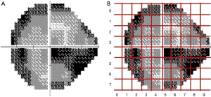
M is the two-dimensional matrix, r is rows number of M, c is the number of the column of M. If M is the matrix of a completely black image, then any value in M is 0, and the calculation result of the formula is 0; if M is for a completely white image, then any value in M is 255, and the calculation result of the formula is 1. It can be seen that the smaller the value is, the more serious the VF damage level is.
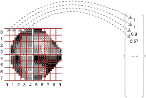
The grayscale training model extracted the data from top to bottom and left to right. The mapping process is shown in Figure 2. The output result is the column vector.
Neural network construction
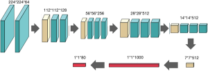
In the training model of the grayscale map inherited from the Visual Geometry Group Network (VGGNet), we used the convolution and pooling layers in the VGG19 model (the 16 hidden layers in front of the VGG19 model) and added two new full connection layers at the end of the model. The neural network is shown in Figure 3.
The loss function of the model was designed to make the vector close to the real sample data value. In our model, we used a Euclidean distance formula to calculate the distance between the predicted vector data of the model and the corresponding sample vector data. The following formula shows the detail of the calculation:
|
| [2] |
V' is the predicted vector data of the model, V is the sample vector data, and n is the result of the dimension value of the vector minus by one (since the dimension value of the vector is counted from 0).
In the real vector, the more non-zero elements in the vector there are, the larger the deviation between the sample vector data and the predicted vector data will be. The improved model follows the Euclidean distance formula. The final distance is divided by the number of non-zero elements in the sample vector data; the updated formula is as follows:
|
| [3] |
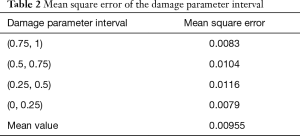
Approximately 10% of the reliable samples were randomly selected to test the model performance. The AI model predicted the damage parameters for each grid of the grayscale map and calculated the mean square error (MSE) of the predicted values and the grayscale values. Finally, the AI model test obtained the MSE in different damage parameter intervals.
Structure data transformation
Assuming V is the output vector data of the model, the index i element V[i] can get its x and y dimension value by the following formula:
|
| [4] |
Where h is the height of the grid, and w is the weight of the grid, then the range-box of G<x,y> can be calculated by the following formula:
|
| [5] |
Where xstart is the start value of the horizontal coordinate in the range-box, ystart is the start value of the vertical coordinate in the range-box, wa is weight value of the range-box, and ha is height value of the range-box. Moreover, the range-box data can be obtained directly by the order number of vector with the following formula:
|
| [6] |
Ultimately, the quintuple data T(V[i]) can be obtained by the following formula:
|
| [7] |
In the quintuple data, the attribution of the “level” is to record the VF damage parameters in the corresponding grid. After model processing, the quintuple data sets can be retrieved from each input image to represent the damage status of the VF, and can used for visual simulation in patients.
Visual simulation
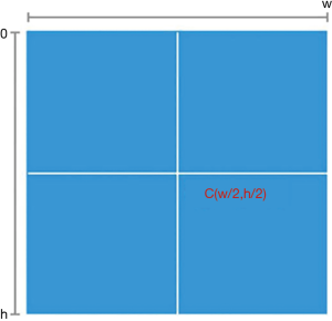
For the visual stimulation by mapping the VF damage parameters into the real scene image, we needed to transform the center point once the resolution of the real scene image was larger than that of the VF check result image (450*400). The definition of the center point is shown in Figure 4; h is the height value of the image, w is weight value of the image, and the coordinate of the center point is (w/2,h/2). The transformation process is shown in Figure 5; the VF check result image is the same as the center point of the real scene image after the transformation.
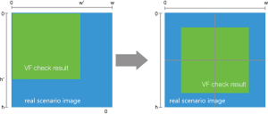
During the transformation of the center point, the attribution of xstart and ystart in the quintuple data will be changed while other attributions remain unchanged. Assuming h is the height value of the real scene image, w is the weight value of the real scene image, h' is the height value of the VF check result image, and w' is weight value of the VF check result image. The attribution of xstart and ystart in the quintuple data can then be recalculated by the following formulas:
|
| [8] |
|
| [9] |
After the center point transformation for all quintuple data, the VF check result image and the real scene image had the same center point, and we then resized the range of the area represented by the quintuple data. Assuming r is the view range value of the real scene image and r' is the view range value of the VF check result image, the resize rate can be calculated by the following formula:
|
| [10] |
We then used the value to recalculate the attributions in quintuple data by the following formulas:
|
| [11] |
|
| [12] |
|
| [13] |
|
| [14] |
After the recalculation for the attributions in quintuple data, we created an initial matrix, with each value of the matrix being 1. The three channels in the matrix are shown in Figure 6A. Next, we mapped the quintuple data into the matrix by filling the attribution value of “level” in the quintuple data into the corresponding place. We had two quintuples as follows:
|
| [15] |
|
| [16] |
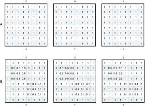
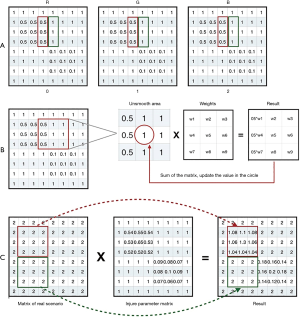
The mapping results of these quintuples are shown in Figure 6B. We named the mapping result as the damage parameters matrix. After completing the visual contour construction based on VF damage parameters, we merged the VF damage parameters matrix with the matrix of the real scene image to simulate the VF damaged area in the real scenario. The damage parameters matrix in Figure 7A used Gaussian smoothing filtering. Since three channels were the same, one of them used a representative example; the process is shown in Figure 7B. After the filtering, the apparent boundary between the damaged area and the background was eliminated, while most of the background values remained “1”. The filtering process does not change the value of the VF normal area in the real scene image, as shown in Figure 7C.
Clinical validation
This study’s clinical validity was divided into two parts: the pilot study and clinical trial. The pilot study mainly used the sample size estimation. In the pilot study, 10 groups of HVF grayscale maps were randomly selected from reliable samples of VF defects, and 10 groups of AI simulations were generated accordingly. The value of the gray value of the image ranged from 0 to 10: 0 indicated the VF was normal, and 10 indicated the VF was seriously damaged. The image was divided into 80 grids, and the gray value of each grid was calculated as follows:
|
| [17] |
M is a two-dimensional pixel matrix of the grayscale expression mode of the grid, r is the number of rows of the matrix, and c is the number of columns of the matrix. After calculating the cumulative gray value of these images, SPSS 25.0 was used to test the statistical difference between the HVF grayscale map and AI simulations. The sample size in the clinical trial was calculated by using the following two-sample mean comparison formula:
|
| [18] |
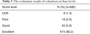
n1 and n2 are the required contents of the two samples, respectively. δ is the difference between the population mean values, σ is the population standard deviation, and uα and uβ are the u values related to the detection level α and type II error probability β (the unilateral test level α is 0.05, and β is 0.1). The clinical trial was divided into two parts: the comparison of the cumulative gray value and the analysis of the shape-position matching degree. After the pilot study calculated the sample size, the clinical trial was constructed to be a double-blind and equivalence analysis. The HVF grayscale maps and AI simulations were randomly selected as the control group and the test group from the reliable sample data of VF defects. After using the same method as the pilot study to calculate the cumulative gray value of the two groups, the two independent samples t-test were used to test whether there was a statistical difference between the control group and the test group. In the clinical trials of the shape and position matching degree, we enrolled three ophthalmologists as volunteers (Wenwen Ye, Xuelan Chen, and Hongli Cai) with normal VF. The volunteers were asked to score the shape and position between the two groups from 0 to 100, with 0 indicating a complete mismatch, and 100 indicating a perfect match. The average scores of three volunteers were calculated in each group of images and divided into four levels as follows: 0–25, unfit; 26–50, poor; 51–75, good; 76–100, excellent. After the group of images was scored, the ratio of the four levels was calculated, and the ratio of the good and the excellent was considered the shape and position matching rate.
Results
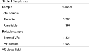
We collected 3,660 VFs of the 24-2 strategy for AI model training. Among them, the reliable samples consisted of 1,334 normal VFs and 1,929 VF defects that met the criteria of the reliability indices (Table 1).
Full table
In the process of AI model training, we first divided the grayscale map into 80 equal-sized grids according to the model algorithm and performed feature extraction analysis on each grid to obtain feature parameters. The feature parameters were then calculated by each grid to generate vectors as intermediate outputs. Finally, the area coordinates and VF damage information were converted into the result vectors. Since each grid of the grayscale map had no fixed features, assigning them could not be done directly. By calculating the average degree of darkening in each grid, the damage type parameter could be obtained.
The performance of the AI model was validated, and the results of 311 grayscale map test samples were predicted. The MSE of the damage parameter interval in the predicted values and the grayscale values are shown in Table 2. The MSE in the (0.75, 1) and (0, 0.25) intervals was less than that in the (0.5, 0.75) and (0.25, 0.5) interval.
Full table
In computer vision processing, the area and damage information in the VF damage parameter quintuple data set were mapped into the real scene image, and the darkening effect was adjusted according to the damage parameter; the visual effects in patients were thus simulated into the real scene image. After constructing the visual contour based on the VF damage parameter, the visualization matrix of the VF damaged area and the real scene images processed by the Gaussian smoothing filter were merged.
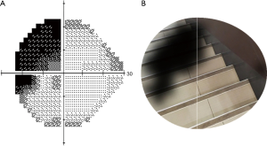
The grayscale map of VF defects was input into the model, and the real scene image was selected from a stairs picture. After processing by computer vision technology, the AI model preliminarily simulated the monocular visual effects in patients with VF defects, as shown in Figure 8.
Clinical validation results
The SPSS statistical results in the pilot study are shown in Table 3. After statistical analysis, the Levene Variance Equality Test indicated that the two groups had the same variance (F value =0.174, P=0.782), and two independent samples t-test indicated that there was no statistical difference between the groups (t=0.379, P=0.709). Based on the pilot study, the overall mean difference δ was taken as 13, and the standard deviation of the AI simulations was used instead of the total standard deviation σ=74. After checking the u-value list (uα=1.96. uβ=1.282), the sample size of the control group and the test group was 682.

Full table
The SPSS statistical results of the clinical trial are shown in Table 4. The cumulative gray values between the HVF grayscale map and the AI VF simulation were similarly analyzed, and the difference was not statistically significant. After the evaluation was complete, each group’s average score was divided into four groups. The proportion of excellent and good levels was 96.0%, as shown in Table 5.

Full table
Full table
Discussion
We developed an AI model based on the grayscale map in the 24-2 VF strategy by using DL and computer vision technology. In the real scenario, the AI model could preliminarily simulate patients’ monocular VF effects of 24°, in which the nasal VF extended to 30°.
VF defect diseases can severely impact patients’ quality of life (21), and glaucoma, a type of this condition, has become the second most common eye disease in the world even when over half of the glaucoma patients in developed countries are estimated to have not been diagnosed (22). The prevalence of glaucoma in China is about 3%. However, 80% of glaucoma patients are misdiagnosed, especially in rural areas (23-25). Therefore, the VF test is an important indicator, one version of which, HFA, is commonly used as perimetry to diagnose and observe VF defects (26-28).
In this study, we used the 24-2 strategy in HFA, in which the nasal side extends to 30° of VF. Other research has used the 30-2 strategy to study VF defects (16), in which the depth and range of the VF defects would be more severe than the 24-2 strategy because of the longer test time, potentially causing psychological fatigue and visual stress (29). Thus, many medical institutions regard the 24-2 strategy as the standard procedure because of the minimal diagnosis time involved (30).
In our study, the grayscale map was chosen to train the AI model. For many clinicians who have not received any HFA-related training, they have difficulties in diagnosing the VF by analyzing the statistical chart in HVF test results. The threshold values reflect the decibel sensitivity at each tested point, which cannot directly and quickly explain the test result. The total deviation map is mainly used to correct the patient’s age factor, and the pattern deviation map corrects the effects of refractive interstitial opacity and other conventional VFs (31).
The grayscale map was based on the actual light sensitivity value of each tested point in the HFA. The grayscale map can intuitively reflect the VF test results by converting the light threshold into grayscale (32). The grayscale map can be used to diagnose the VF defects of patients more quickly and intuitively, and thus the clinician without HFA training can also have a preliminary judgment on the VF test result. The VF defects in glaucoma are irreversible, but the patient may not perceive the monocular VF change due to the binocular compensation (33). The grayscale map can help clinicians to diagnose the patient’s visual condition in good time, and to prevent the possible delay of patient’s treatment.
We used the VGGNet network structure to build our AI model, which was a CNN developed by researchers at the Visual Geometry Group of Oxford University and Google DeepMind (34). VGGNet has two structures: VGG16 and VGG19. Compared to traditional CNN, the application of VGGNet has a profound influence on DL (35). VGG19 adopts the alternating structure of multiple convolutional layers and nonlinear activation layers, which improves the network depth and extracts image features more effectively than a single convolutional layer structure (36,37). Since the image in each grid of the grayscale map has no fixed features, it cannot be directly assigned. By calculating the average gray values in each grid, the damage type parameter can be obtained. After the construction of the AI model, visual processing is required to transform the data into the real scene. After the visual contour construction based on VF damage parameters was completed, the visual matrix of the VF damaged area and the real scene image were required to be processed with a Gaussian smoothing filter. If smoothing is not performed in AI simulations, the image generated by the initialization matrix will have a distinct segmentation edge between the original background and VF damaged area, thus affecting the simulated effect after fusion (38-40).
After constructing the AI model, the model predicted the damage parameters of the grayscale map in the test sample and calculated the MSE between the predicted value and the real value. The MSE showed a downtrend in the (0.75, 1) and (0, 0.25) intervals (MSE =0.0083 and 0.0079) compared to the (0.5, 0.75) and (0.25, 0.5) intervals (MSE =0.0104 and 0.0116). The results indicated that the AI model had a higher prediction accuracy in the normal VF and VF defects area in the grayscale map.
In order to test the AI simulation of the patient’s VF defects in the real scenario, we conducted the clinical validation of the AI model. There are very few comparisons of the cumulative gray values between the grayscale map and an AI simulation reported in the literature. Therefore, to ensure the sample size of this clinical trial, a pilot study was carried out to obtain sufficient statistical performance. In clinical trials, since the AI simulation is based on the HVF grayscale maps, the cumulative gray values have partial results if the statistical method uses the paired t-test. Therefore, using the two independent sample t-test is more in line with this clinical trial. After analyzing two independent sample t-test (t=1.317, P=0.188, P>0.05), the difference was not statistically significant. The results indicated that the patients with VF defects were consistent with the area of bright and shade between the AI simulation and the grayscale map. For validating the consistency of the shape and position between the grayscale map and the AI simulation, we enrolled three volunteers ophthalmologists to score the shape and position between the two groups. Background in ophthalmology and double-blind evaluations reduced the risk of bias (41). A total of 615 cases received excellent scores, and the combined rate of good and excellent grades reached 96%. The three ophthalmologists approved of our AI simulation. In the future, our AI simulations may help clinicians reduce the misdiagnosis of patients with VF defects in real practice.
Our study has some limitations. The simulation of visual effects was performed only based on the patient’s VF test results and exclusive of other influencing factors such as visual acuity, color vision, and contrast sensitivity. Therefore, in a future study, we plan to add vision-related data including vision, color vision, and contrast sensitivity for model training, thereby obtaining a more comprehensive visual function parameter.
Conclusions
In summary, based on the 24-2 strategy commonly used in the VF test, this study developed an AI VF model, which could simulate the visual effects of patients with VF defects in real practice; the monocular VF was 24°, in which the nasal extended to 30°. The AI simulation will help clinicians, patients, and patient families to understand the HVF test results. Our findings can help lay a foundation for subsequent research and the health education related to visual impairment and rehabilitation.
Acknowledgments
Thanks are due to Dr. Haotian Lin, the Director of Department of Artificial Intelligence and Big Data Department of Zhongshan Ophthalmic Center of Sun Yat-sen University for advice on experimental design. And thanks Wenwen Ye, Xuelan Chen, and Hongli Cai from The Second Affiliated Hospital of Fujian Medical University for assistance with the experiments.
Funding: This work was supported by the National Key R&D Program of China Sub-project Fund for Scholars (award number: 2018YFC0116500 and 2018YFC2002600) and Sanming Project of Medicine in Shenzhen (No. SZSM201812090).
Footnote
Provenance and Peer Review: This article was commissioned by the Guest Editors (Haotian Lin and Limin Yu) for the series “Medical Artificial Intelligent Research” published in Annals of Translational Medicine. The article was sent for external peer review organized by the Guest Editors and the editorial office.
Conflicts of Interest: All authors have completed the ICMJE uniform disclosure form (available at http://dx.doi.org/10.21037/atm.2020.02.162). The series “Medical Artificial Intelligent Research” was commissioned by the editorial office without any funding or sponsorship. The authors have no other conflicts of interest to declare.
Ethical Statement: The authors are accountable for all aspects of the work in ensuring that questions related to the accuracy or integrity of any part of the work are appropriately investigated and resolved. The Ethical Review Committee approved the study of Shenzhen Eye Hospital Affiliated to Jinan University (approval number: 201009031). Studies involving human subjects were conducted following the Helsinki Declaration.
Open Access Statement: This is an Open Access article distributed in accordance with the Creative Commons Attribution-NonCommercial-NoDerivs 4.0 International License (CC BY-NC-ND 4.0), which permits the non-commercial replication and distribution of the article with the strict proviso that no changes or edits are made and the original work is properly cited (including links to both the formal publication through the relevant DOI and the license). See: https://creativecommons.org/licenses/by-nc-nd/4.0/.
References
- Yohannan J, Wang J, Brown J, et al. Evidence-based Criteria for Assessment of Visual Field Reliability. Ophthalmology 2017;124:1612-20. [Crossref] [PubMed]
- Liu GT, Volpe NJ, Galetta SL. Visual Loss: Overview, Visual Field Testing, and Topical Diagnosis In: Liu GT, Volpe NJ, Galetta SL. editors. Liu, Volpe, and Galetta's Neuro-Ophthalmology. 3rd edition. Elsevier, 2019:39-52.
- Yarmohammadi A, Zangwill LM, Diniz-Filho A, et al. Relationship between Optical Coherence Tomography Angiography Vessel Density and Severity of Visual Field Loss in Glaucoma. Ophthalmology 2016;123:2498-508. [Crossref] [PubMed]
- Corbetta M, Ramsey L, Callejas A, et al. Common behavioral clusters and subcortical anatomy in stroke. Neuron 2015;85:927-41. [Crossref] [PubMed]
- Duncan JE, Freedman SF, El-Dairi MA. The incidence of neovascular membranes and visual field defects from optic nerve head drusen in children. J AAPOS 2016;20:44-8. [Crossref] [PubMed]
- Kanski JJ. Clinical ophthalmology: a synopsis, 2nd edition. Elsevier Health Sciences, 2009.
- Beck RW, Bergstrom TJ, Lichter PR. A clinical comparison of visual field testing with a new automated perimeter, the Humphrey Field Analyzer, and the Goldmann perimeter. Ophthalmology 1985;92:77-82. [Crossref] [PubMed]
- Artes PH, Iwase A, Ohno Y, et al. Properties of perimetric threshold estimates from Full Threshold, SITA Standard, and SITA Fast strategies. Invest Ophthalmol Vis Sci 2002;43:2654-9. [PubMed]
- Lee A, Taylor P, Kalpathy-Cramer J, et al. Machine Learning Has Arrived! Ophthalmology 2017;124:1726-8. [Crossref] [PubMed]
- Lee CS, Baughman DM, Lee AY. Deep learning is effective for the classification of OCT images of normal versus Age-related Macular Degeneration. Ophthalmol Retina 2017;1:322-7. [Crossref] [PubMed]
- Lee CS, Tyring AJ, Deruyter NP, et al. Deep-learning based, automated segmentation of macular edema in optical coherence tomography. Biomed Opt Express 2017;8:3440-8. [Crossref] [PubMed]
- Krizhevsky A, Sutskever I, Hinton GE, et al. ImageNet Classification with Deep Convolutional Neural Networks. Neural Information Processing Systems 2012:1106-14. Available online: https://dblp.org/rec/conf/nips/KrizhevskySH12
- Zeiler MD, Fergus R. Visualizing and Understanding Convolutional Networks. In: Fleet D, Pajdla T, Schiele B, et al. editors. European conference on computer vision. Cham: Springer, 2014:818-33.
- Sermanet P, Eigen D, Zhang X, et al. Overfeat: Integrated recognition, localization and detection using convolutional networks. arXiv:1312.6229, 2013.
- Simonyan K, Zisserman A. Two-Stream Convolutional Networks for Action Recognition in Videos. arXiv:1406.2199, 2014.
- Asaoka R, Murata H, Iwase A, et al. Detecting Preperimetric Glaucoma with Standard Automated Perimetry Using a Deep Learning Classifier. Ophthalmology 2016;123:1974-80. [Crossref] [PubMed]
- Li F, Wang Z, Qu G, et al. Automatic differentiation of Glaucoma visual field from non-glaucoma visual filed using deep convolutional neural network. BMC Med Imaging 2018;18:35. [Crossref] [PubMed]
- Wang M, Shen LQ, Pasquale LR, et al. An Artificial Intelligence Approach to Detect Visual Field Progression in Glaucoma Based on Spatial Pattern Analysis. Invest Ophthalmol Vis Sci 2019;60:365-75. [Crossref] [PubMed]
- Yousefi S, Kiwaki T, Zheng Y, et al. Detection of Longitudinal Visual Field Progression in Glaucoma Using Machine Learning. Am J Ophthalmol 2018;193:71-9. [Crossref] [PubMed]
- Wen JC, Lee CS, Keane PA, et al. Forecasting future Humphrey Visual Fields using deep learning. PLoS One 2019;14:e0214875. [Crossref] [PubMed]
- Medeiros FA, Gracitelli CP, Boer ER, et al. Longitudinal changes in quality of life and rates of progressive visual field loss in glaucoma patients. Ophthalmology 2015;122:293-301. [Crossref] [PubMed]
- Quigley HA. Glaucoma. Lancet 2011;377:1367-77. [Crossref] [PubMed]
- Liang YB, Friedman DS, Zhou Q, et al. Prevalence of primary open angle glaucoma in a rural adult Chinese population: the Handan eye study. Invest Ophthalmol Vis Sci 2011;52:8250-7. [Crossref] [PubMed]
- Wang YX, Xu L, Yang H, et al. Prevalence of glaucoma in North China: the Beijing eye study. Am J Ophthalmol 2010;150:917-24. [Crossref] [PubMed]
- He M, Foster PJ, Ge J, et al. Prevalence and clinical characteristics of glaucoma in adult Chinese: a population-based study in Liwan District, Guangzhou. Invest Ophthalmol Vis Sci 2006;47:2782-8. [Crossref] [PubMed]
- Allingham RR, Damji KF, Freedman SF. editors. Shields textbook of glaucoma. 6th edition. Lippincott Williams & Wilkins, 2012.
- Wang M, Pasquale LR, Shen LQ, et al. Reversal of Glaucoma Hemifield Test Results and Visual Field Features in Glaucoma. Ophthalmology 2018;125:352-60. [Crossref] [PubMed]
- Fallon M, Valero O, Pazos M, et al. Diagnostic accuracy of imaging devices in glaucoma: A meta-analysis. Surv Ophthalmol 2017;62:446-61. [Crossref] [PubMed]
- Asman P, Heijl A. Glaucoma Hemifield Test. Automated visual field evaluation. Arch Ophthalmol 1992;110:812-9. [Crossref] [PubMed]
- Tan NYQ, Tham YC, Koh V, et al. The Effect of Testing Reliability on Visual Field Sensitivity in Normal Eyes: The Singapore Chinese Eye Study. Ophthalmology 2018;125:15-21. [Crossref] [PubMed]
- Katz J. A comparison of the pattern- and total deviation-based Glaucoma Change Probability programs. Invest Ophthalmol Vis Sci 2000;41:1012-6. [PubMed]
- Rowe F. Visual fields via the visual pathway. 2nd edition. Crc Press, 2016.
- Sharma P, Sample PA, Zangwill LM, et al. Diagnostic tools for glaucoma detection and management. Surv Ophthalmol 2008;53 Suppl1:S17-S32. [Crossref] [PubMed]
- Simonyan K, Zisserman A. Very deep convolutional networks for large-scale image recognition. arXiv:1409.1556, 2014.
- LeCun Y, Bengio Y, Hinton G. Deep learning. Nature 2015;521:436. [Crossref] [PubMed]
- Shin HC, Roth HR, Gao M, et al. Deep Convolutional Neural Networks for Computer-Aided Detection: CNN Architectures, Dataset Characteristics and Transfer Learning. IEEE Trans Med Imaging 2016;35:1285-98. [Crossref] [PubMed]
- He K, Zhang X, Ren S, et al. Deep Residual Learning for Image Recognition. computer vision and pattern recognition. 2016 IEEE Conference on Computer Vision and Pattern Recognition (CVPR), Las Vegas, NV, 2016:770-8. doi: [Crossref]
- Laverick KT, Chantasri A, Wiseman HM. Quantum State Smoothing for Linear Gaussian Systems. Phys Rev Lett 2019;122:190402. [Crossref] [PubMed]
- Strappini F, Gilboa E, Pitzalis S, et al. Adaptive smoothing based on Gaussian processes regression increases the sensitivity and specificity of fMRI data. Hum Brain Mapp 2017;38:1438-59. [Crossref] [PubMed]
- Lopez-Molina C, De Baets B, Bustince H, et al. Multiscale edge detection based on Gaussian smoothing and edge tracking. Knowledge-Based Systems 2013;44:101-11. [Crossref]
- Mimouni M, Krauthammer M, Gershoni A, et al. Positive Results Bias and Impact Factor in Ophthalmology. Curr Eye Res 2015;40:858-61. [Crossref] [PubMed]

