
Decision curve analysis: a technical note
Introduction
Decision curve analysis (DCA) has been increasingly being used for the assessment of diagnostic tests and/or prediction models in clinical researches. The advantage of DCA is that it integrates the preferences of the patients or policy makers into analysis. Traditional metrics of diagnostic performance such as sensitivity, specificity and area under receiver operating characteristic curve (AU-ROC) only measure the diagnostic accuracy of one prediction model against another, but fail to account for the clinical utility of a specific model (1).
DCA was developed to overcome this problem. A key concept of DCA is the threshold probability, which was defined in the seminal paper by Vickers AJ that “threshold probability, pt, is where the expected benefit of treatment is equal to the expected benefit of avoiding treatment.” (2). In definition, it is obvious that the threshold probability can vary from patient to patient. For example, surgery-averse patients may opt to take surgery at a high risk of cancer, but cancer-averse patients are more likely to perform operation at lower risk of cancer. Thus, the DCA allows threshold probability to vary to examine whether one model is superior to another at a certain range of threshold probability (3), with respect to “the net benefit”. In this technical note, we provide code to implement DCA in an R environment, including plotting the net benefit, correction for overfitting, confidence intervals and a statistical test to compare two models over a range of threshold probabilities. Before providing our routines, we start by briefly recalling the concept of net benefit.
Concept of net benefit
Suppose that we have developed two models to predict/diagnose a disease, such as sepsis; then every patient can have a predicted probability of sepsis (pi) based on one of the models. The rationale is that patients with pi > pt are judged as positive and will be treated and those with pi < pt are judged negative and will not be treated.
To compare two models at a given threshold probability, the key concept of DCA is to calculate the net benefit (for the treated) with the following equation (2):
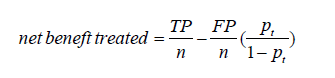
where TP and FP are true positive count and false positive count, respectively; n is the number of subjects; and pt is the threshold probability. A model is said to be superior to another at the chosen threshold probability pt if its net benefit surpasses the net benefit of the other model for that value of pt. The two models can also be compared to the two extreme strategies of treating all the patients [where TP/n = π and FP/n =1–π in the equation above, π = (TP + FN)/n being the prevalence of the disease, i.e., the event rate] and of treating none of the patients (where TP = 0 and FP = 0 the net benefit being thus 0 at any threshold probability).
That computation of the net benefit is based on treated patients. One could similarly calculate a net benefit based on untreated patients. The net benefit for the untreated patients can be expressed as a function of pt as follows (4):
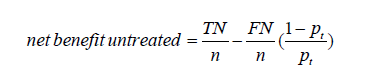
where TN and FN are true negative count and false negative count. One will get here TN = 0 and FP = 0 (and a net benefit of 0 at any threshold probability) for the strategy of treating all the patients, and TN/n = 1–π and FN/n = π for the strategy of treating none of the patients.
Interestingly, one can check that we have the following relationship between the concept of the net benefit for treated and untreated patients as follows:
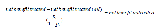
where net benefit treated (all) = π – (1–π)pt/ (1-pt) refers to the net benefit for the treated calculated for the extreme strategy of treating all the patients, as mentioned above. When multiplied by 100, Vickers and Elkin (2) interpreted this quantity (which thus turns out to be what has then been called the net benefit for the untreated) as the number of avoidable treatments (identified thanks to the model) in 100 patients who would be otherwise treated, which is “net of false negative”. Similarly, the net benefit for the treated could be interpreted as the number of profitable treatments (identified thanks to the model) in 100 patients who would be otherwise left untreated, which is “net of false positive”.
Finally, one could focus on both the treated and the untreated patients and calculate the “overall net benefit” by summing up the net benefit for the treated and the untreated (4):

Note that while the difference of the net benefit achieved by two models will differ whether focusing on the treated, the untreated or overall, the ranking of models w.r.t. to the net benefit will remain the same for each of these three definitions.
More recently, Lee and Wu proposed the average deviation about the probability threshold (ADAPT) index for determining the utility of a prediction model, which can be calculated as follows (5):
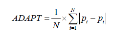
Interestingly, at least when the model is correctly calibrated (i.e., when the predicted probabilities pi really correspond to the probabilities of having the disease), one can show that (5):

Working example
An artificial data set is simulated for the illustration purpose. There is no clinical relevance of the simulated dataset.

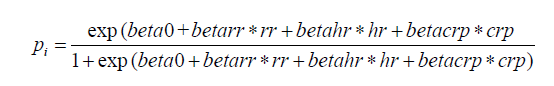
The above code generated a data frame containing 4 variables: respiratory rate (rr), heart rate (hr), C-reactive protein (crp) and observed disease status (sepsis.tag). The first three variables will be the predictors and the last one (sepsis) will be the response (outcome) to be predicted. For simplicity, note that no correlation has been generated among the three predictors. The probability pi to have sepsis has thus been generated as:
Such a model with three predictors will be referred to as the “full model” in what follows, which shall be compared with a “simple model” including only the former two predictors.
Net benefit function
R code to perform DCA has been well described in the website: https://www.mskcc.org/departments/epidemiology-biostatistics/health-outcomes/decision-curve-analysis-01. However, the dca() function provided in the website generated prediction models for one predictors at a time and it requires each predictor to be transformed to the probability scale (ranging from 0 to 1). In some situations, investigators may want to create a model with a number of predictors. Here, we create a new function to calculate net benefits at varying values of threshold probability. This function also allows to calculate the different kinds of net benefits mentioned above (treated, untreated, overall or the ADAPT index).

There are nine arguments in the ntbft() function:
- data: a data frame on which the prediction model is trained.
- outcome: a character string indicting the name of the outcome or disease status.
- frm: a formula in the form of outcome~predictor 1 + predictor 2, where each variable should be the contained in the data frame. The argument specifies the prediction model to be fitted in case the argument pred below is NULL (if the pred argument is provided, frm is not used).
- exterdt: a data frame to specify whether the prediction should be made in external dataset; this is useful for cross validation of the model. By default, the value is NULL, indicating the prediction is made in the same dataset as the training dataset.
- pred: a vector of predicted values to be used to calculate the net benefit. By default, the value is NULL, indicating that such predicted values should be calculated by the routine using the model specified by frm.
- xstart: the starting point of the threshold probability, the default value is 0.01.
- xstop: the end point of the threshold probability, the default value is 0.99.
- step: a numerical value specifying the incremental step of the threshold probability, the default value is 0.01.
- type: controls the type of net benefit to be computed. The allowed values correspond to the treated (“treated”), untreated (“untreated”) and overall (“overall”) patients, or to the ADAPT index (“adapt”). The default is the “treated”.
The returning object of the ntbft() function is a data frame containing 4 columns: threshold, all, none and pred. The “threshold” column is a column containing threshold probability at which net benefit will be calculated. “all” column is the net benefit for treating all patients, and “none” column is the net benefit for treating none patients. The “pred” column contains net benefit values for treating patients by using the prediction model.
Plotting the net benefit of a simple and a full model
Sepsis can be predicted by simply using vital signs such as heart rate (hr) and respiratory rate (rr), which is cheap and easy to perform (simple model). Laboratory test such as crp is costly but can help to increase the predictive accuracy (full model). The net benefit for these two models can be calculated as follows (the starting point, the end point and the incremental step of the threshold probabilities, as well as the type of net benefit to be considered can be changed by the user if one wishes):

The results can be visualized by using ggplot2 system (6). A dedicated routine to plot the net benefit of different models is provided below, where it is convenient to reshape the data frame, aggregating all net benefit values in one column (7). Such a long format dataset can be easily mapped to the coordinate system with groups.

There are six arguments in the plot.ntbft() function:
- nb: a data frame of net benefit, where the first column contains the threshold probabilities and the next columns contains the net benefit achieved for different models.
- nolines: the number of the columns of nb which should be plotted using lines. The default is to plot all columns (except the first one containing the threshold).
- nobands: the number of the columns of nb which should be plotted using bands (useful to plot confidence intervals). The default is to plot no bands.
- ymin: the minimum of net benefit to be plotted. The default is −0.1.
- ymax: the maximum of net benefit to be plotted. The default is the maximum of the net benefits which are plotted either via lines or via bands.
- legpos: a vector of two coordinates indicating where the legend should be in the graph.
One can then plot the net benefit of the two above models on the same graph as follows:

The output of the above example is shown in Figure 1. The net benefit is plotted against the threshold probability. The “all” line shows the net benefit by treating all patients, and the “none” line is the net benefit for treating none patients. It appears that the full model is always superior to the simple model across a wide range of threshold probabilities, with the highest difference at a threshold probability around 0.5. At that threshold, the net benefit (for the treated) is 0.030 for the simple model, and 0.162 for the full model. At that threshold, according to the interpretation given above, this means that one can administrate about 16−3=13 more profitable treatments (out of 100 patients) when using the full model rather than the simple model to predict sepsis (net of false positive).

Bootstrap method to correct overfitting
In the above example, the model training and prediction were performed in the same dataset, which can cause the problem of overfitting. The overfitting can be corrected by using bootstrap resampling method with the following steps (8):
- Sample with replacement from the original dataset;
- Fit a model with the sample generated in step 1;
- Use the fitted model in step 2 to predict probability of the event of interest in the bootstrap sample, and then calculate net benefit at various threshold probabilities;
- Use the fitted model in step 2 to predict probability of the event of interest in the original dataset, and then calculate net benefit at various threshold probabilities;
- Compute the difference in net benefit obtained by step 3 and 4;
- Step 1 to 5 is repeated for a number of times [500], and mean difference in net benefit across the 500 times can be computed.
- The uncorrected net benefit minus the mean difference obtained in step 6 gives the corrected net benefit.
Before conducting bootstrap replicates, we first need to define a function to calculate the difference of net benefit (or over-optimism) of the net benefit obtained when evaluated on the same or a different data set as that used to train the model.

Five out of the 6 arguments of the diffnet() are the same as that in the ntbft() function. The argument ii to allow boot() function to select a sample, frm to specify the model formula and outcome to specify the response variable. The function returns a data frame containing the difference of net benefit as described in step 5 of the algorithm above. One can then apply the following code to correct overfitting for our simple model and to plot the result obtained:

The boot() function is employed to perform the bootstrap procedure. In the example, the statistic argument specifies a function that returns a vector containing the statistic(s) of interest; a total of R=500 bootstrap replicates have been performed (but the user could easily change this parameter). Then, the corrected net benefit is computed by subtracting the mean difference from the net benefit estimated with the simple model. The obtained result is plotted in Figure 2. It shows that the corrected net benefit is very close to the uncorrected one, suggesting the overfitting is not a serious problem in our example. This is not surprising because the covariates are independent to each other and there is no noise factor (no overfitting). If correlated or noise covariates are included in the model, it may not be the case.

Cross validation to correct overfitting
An alternative to bootstrap to assess overfitting is cross-validation, or out-of-sample validation, which is widely used for model validation. One round of cross-validation involves splitting the original dataset into complementary subsets, performing the analysis on one subset (called the training set), and validating the analysis on the other subset (called the validation set or testing set). It is common to perform multiple rounds of cross-validation using different partitions, and the validation results are averaged over the rounds to give an estimate of the model’s predictive performance. In our situation, the cross-validation is performed in following steps (8):
- The original sample is randomly split into k (e.g., k=10) equal sized subsets;
- Fit the model with k-1 subsets by leaving out the first subset;
- Predicted probability is obtained by applying the fitted model to the first subset;
- Repeat steps 2 and 3 by leaving out and then apply the fitted model to the ith group for i = 2,3,.., k–1, k. After these procedures, every patient has a predicted probability for the outcome of interest.
- The predicted probability is then used to calculate net benefit as described above.
- Bootstrap the above steps for a number of times (e.g., 200) and the corrected net benefit is the mean of these bootstrap results.
Here would be a function to perform cross-validation:

Seven out of the 9 arguments of the diffnet() are as in the ntbft() function. The argument n_folds specifies the number of k folds to split the original dataset (default is 10) and the argument R specifies the number of bootstrap replicates (default is 200), as described in the algorithm above. The function returns the cross-validates net benefit. One can then apply the following code to cross-validate our simple model and to plot the result obtained:

The obtained result (using 10 folds cross-validation and 200 replicates) is plotted in Figure 3, which again shows that overfitting is not a serious problem in our example.

Confidence interval for the decision curve
Confidence interval of a statistic can be estimated using bootstrap method. Firstly, we define a function for computing the net benefit (with exactly the same arguments as the function diff.net above):

Calculation of 95% confidence interval for the net benefit of our simple model based on R=500 bootstrap replications, together with a plot of the results can then be obtained as follows:

The output Figure 4 shows the confidence interval for the decision curve of our simple model.

Comparing two decision curves and reporting P value
A test to compare two decision curves (obtained using two different models) can also be performed via bootstrap. Firstly, we define a function for comparing to such models.

The nbdiff() function computes the difference of net benefit for two models. The competing models are defined by frm1 and frm2. One can then compare our simple and full models as follows (using 500 bootstrap replications):

It turns out that the two models significantly differ at the 5% level for 64 threshold probabilities (all lying between 0.06 and 0.72) while they did not significantly differ at the remaining 35 thresholds (either below 0.06 or higher than 0.72).
Trapezoidal numerical integration
The above method provides a pointwise comparison (e.g., one P value for each threshold probability) between decision curves of two competing models. However, in some situations one would like to have a single (global) P value to compare two models over a range of threshold probabilities. Area under the net benefit curve (A-NBC) is a summary statistic for the performance of the model in the range of threshold probabilities of interest. This method is criticized for not considering the fact that the threshold probabilities are not uniformly distributed in the range of interest (9,10). However, we proposed that this will be valid for a small range of pt. Here, we present the method for comparing A-NBCs of two models using trapezoidal numerical integration. In mathematics, and more specifically in numerical analysis, the trapezoidal rule (also known as the trapezoid rule or trapezium rule) is a technique for approximating the definite integral. The trapezoidal rule works by approximating the region under the graph of the function f(x) as a trapezoid and calculating its area. The difference in the trapezoidal area of two NBCs is the statistic of interest.

The areadiff() function has several arguments, most of them are similar to that described in previous sections. Here the xstart and xstop arguments define the range of interest. Then, we use the boot() function to replicate the difference in the A-NBCs. For example, we can compare our simple and full model using 1,000 bootstrap replications over the threshold range 0.01–0.1 as follows:

The result shows that the P value for the difference in A-NBC between in the threshold range from 0.01 to 0.1 is 0.021 (we have thus a significant difference between the two models on that threshold range).
The ADAPT index
The ADAPT values obtained by the all and null models are used as the boundary for the competing models. The following R code generates ADAPT curve for the models in our example (Figure 5).


The rmda package
The rmda (previously called DecisionCurve) package is well suited for the purpose of drawing decision curves (11). It is different from our routines in several aspects: (I) the rmda package allows display of the cost:benefit values at the bottom of the decision curve plot, which corresponds to relevant threshold probability values; (II) it reports the standardized net benefit; (III) it provides functions for alternative plots showing measures of clinical impact or the components of the ROC curve (true/false positive rates) across a range of risk thresholds. However, the rmda package does not allow the calculation of the ADAPT index, and comparing decision curves of competing predictive models.

Figure 6 shows the decision curves for the simple and full models.

 . The preference of the patients and clinicians is implicitly expressed by the threshold probability.
Summary
This article is a technical note showing how to perform DCA with an artificial dataset in R environment. In the decision curve, net benefit is plotted against threshold probability. The decision curve of a model is compared to extreme cases that treating all patients or none. A model is of clinical utility if the net benefit of a model is greater than treating all and none patients. Confidence interval and comparisons of two decision curves can be made using bootstrap method. The comparison of two decision curves can be made at a pointwise fashion that a P value is reported for each threshold probability. Furthermore, the comparisons of two decision curves can be made by using A-NBC within a certain threshold probability range. However, A-NBC is criticized for not considering the uneven distribution of the threshold probability. The weighted area under decision curve is an alternative to address this limitation. Our routines have been illustrated using the concept of net benefit for the treated but they can be equally applied to the net benefit for the untreated, the overall net benefit, or the ADAPT criterion.
Acknowledgements
We would like to thank Prof. Andrew J. Vickers from Department of Epidemiology and Biostatistics, Memorial Sloan-Kettering Cancer Center, for his valuable comments to improve the manuscript.
Funding: Z Zhang received funding from The Public Welfare Research Project of Zhejiang Province (LGF18H150005) and Scientific Research Project of Zhejiang Education Commission (Y201737841); X Qian received funding from Scientific Research Project of Zhejiang Education Commission (Y201738001).
Footnote
Conflicts of Interest: The authors have no conflicts of interest to declare.
References
- Fitzgerald M, Saville BR, Lewis RJ. Decision curve analysis. JAMA 2015;313:409-10. [Crossref] [PubMed]
- Vickers AJ, Elkin EB. Decision curve analysis: a novel method for evaluating prediction models. Med Decis Making 2006;26:565-74. [Crossref] [PubMed]
- Vickers AJ, Van Calster B, Steyerberg EW. Net benefit approaches to the evaluation of prediction models, molecular markers, and diagnostic tests. BMJ 2016;352:i6. [Crossref] [PubMed]
- Rousson V, Zumbrunn T. Decision curve analysis revisited: overall net benefit, relationships to ROC curve analysis, and application to case-control studies. BMC Med Inform Decis Mak 2011;11:45. [Crossref] [PubMed]
- Lee WC, Wu YC. Characterizing decision-analysis performances of risk prediction models using ADAPT curves. Medicine (Baltimore) 2016;95. [Crossref] [PubMed]
- Wickham H. ggplot2: Elegant Graphics for Data Analysis. Houston: Springer International Publishing, 2016.
- Zhang Z. Reshaping and aggregating data: An introduction to reshape package. Ann Transl Med 2016;4:78. [PubMed]
- Vickers AJ, Cronin AM, Elkin EB, et al. Extensions to decision curve analysis, a novel method for evaluating diagnostic tests, prediction models and molecular markers. BMC Med Inform Decis Mak 2008;8:53. [Crossref] [PubMed]
- Talluri R, Shete S. Using the weighted area under the net benefit curve for decision curve analysis. BMC Med Inform Decis Mak 2016;16:94. [Crossref] [PubMed]
- Steyerberg EW, Vickers AJ. Decision curve analysis: A discussion. Med Decis Making 2008;28:146-9. [Crossref] [PubMed]
- Kerr KF, Brown MD, Zhu K, et al. Assessing the Clinical Impact of Risk Prediction Models With Decision Curves: Guidance for Correct Interpretation and Appropriate Use. J Clin Oncol 2016;34:2534-40. [Crossref] [PubMed]

