
Instrumental variable analysis in the presence of unmeasured confounding
Introduction
While randomized controlled trials (RCTs) are able to balance both measured and unmeasured confounders between comparison groups by the mechanism of randomization, observational studies usually suffer from confounding effects. Confounders are variables associated with both the assignment of treatment and the outcome (1). When the distributions of confounders are not balanced between treated and control groups in an observational study, the estimated treatment effect can be biased. Various methods have been commonly used to account for measured confounder such as matching, multivariable regression adjustment, stratification and so on (2). However, these methods cannot address the problem of unmeasured confounding, which is not uncommon in clinical researches.
Instrumental variable (IV) analysis is a method widely used in econometrics and social sciences, to account for unmeasured confounding (3). The IV is a variable associated with the treatment assignment, it affects the outcome only through the exposure and it is independent of confounders (4,5). Angrist and Krueger (1991) and others (3,5) provided a good review of applications of the IV method. One challenge in IV analysis is to choose a good IV in a real clinical study. In this paper, we will suggest a systematic strategy for addressing this challenge and introduce easily implemented step-by-step practical advice to perform IV analyses in real studies. Simulations, R codes and real examples in clinical research with the IV approach will be discussed and compared with regular analyses.
Working example
This study is motivated by a real multicenter study we have. The real study investigated the effectiveness of early enteral nutrition (EN) on recovery (measured by mortality) and medical costs in 410 critically ill patients (age: 64.71±16.93 years; male 64%) enrolled in ten tertiary care hospitals (6,7). Traditionally, critically ill patients start EN feeding gradually and after 48 hours since admission. However, the late adoption of EN feeding may delay the recovery of patients leading to higher mortality and longer hospital stays. Therefore, the multicenter study aimed to evaluate if early EN would improve patients’ recovery and reduce mortality and costs. In stage I of the study between April 2016 and July 2016, the attending physicians at the ten hospitals provided usual care or EN based on their own preference and local guidance. Two hundred and thirty-six patients were enrolled in the first stage. In the training period between August 2016 and September 2016, all the physicians, nurses, and dieticians at the ten hospitals received 2-month training of using standardized EN feeding protocol within 48 hours after admission to the hospital. Then in stage II between September 2016 and January 2017, all the ten hospitals fully implemented the standardized EN feeding protocol. 147 patients were enrolled and received the standardized EN protocol in the second stage.
Early EN feeding was measured as the percentage of actual daily EN feeding accounting for the total daily requirement target. Age and severity of patients’ illness are important predictors known to patients’ recovery and can confound the effect of EN feeding if they are not balanced between the comparison groups (Figure 1). In the EN feeding study, severity of illness was measured by the sequential organ failure assessment (SOFA) score, which ranged from 0–24 points with higher values indicating severer illness. To illustrate the IV analysis, we suppose that patients’ age was known but the severity of illness (SOFA) was not measured. When the important confounder illness severity is not measured, IV methods are very helpful for obtaining consistent estimates for effects of early EN feeding on recovery when a valid and strong IV can be found. In an IV analysis, we first would like to have a variable that satisfies the three key features as an IV: relevance, effective random assumption and exclusion restriction (ER) (8). The stage of the EN feeding study is a change in feeding guideline over time and can serve as a natural IV in this study. Baiocchi et al. [2014] discussed some examples using calendar time as the IV, such as the sharply decreased use of hormone replacement therapy (HRT) in 2002 (8). In the EN feeding study, the stage directly affected the use of standardized EN feeding protocol such that the standardized EN feeding (treatment) was sharply increased in stage II (relevance). The change in the feeding practice occurred in a relatively short period of time after a 2-month training period, and there were no notable changes in other medical practices and medical coding systems during the same time period, so the stage of the study seems independent of unmeasured confounders (effective random assumption) and we don’t expect direct effects of the stage time on recovery other than through its effect on the EN feeding practice (ER).

Given that the stage seems a valid IV, we would like to assess its strength on the choice of different feeding practices (treatment). An IV is weak if it only has a slight impact on the treatment choice. A weak IV may lead to a treatment estimate with large variance and sensitive to a slight departure from the three IV assumptions. In the EN feeding study, approximately 40% and 50% of patients took the EN feeding within 48 hours in stages I and II, respectively. The stage had a big impact on the choice of treatment and should work well as a strong IV.
In this study, mortality and medical cost are binary and continuous outcomes of interest, respectively. We will model the two outcomes with appropriate models.
To illustrate the IV analysis, we generated the data in R (version 3.3.2). As discussed above, we will use stage as the IV and evaluate the effects of percentage of actually EN feeding (“percent”) on mortality (“mort”) and medical costs (“cost”) with age as a measured confounder and severity (“sofa”) as an unmeasured confounder (Figure 1).

Assuming that sofa was not measured in the study, we could estimate the treatment effect with a regular (generalized) linear model with sofa omitted and compare this ordinary estimated effect with the true effect for bias.

The above code fit two models. The mod.true model considers the unmeasured confounder and gives the true effect of percent on mort. The exponentiation of the coefficient of treatment “percent” (−0.97) gives an odds ratio of 0.38, indicating that the increase of one unit of the percentage of EN is associated with lower odds of death. The second model mod.biased omits the unmeasured sofa variable, which is commonly done in observational studies when there are unmeasured confounders. It is shown that the second model overestimates the treatment effect by approximately 20% in linear predictor scale (Table 1). The effect of percent on cost is estimated in the same way:


Full table
The cost is a continuous dependent variable and thus is fitted with linear regression model. While the full model estimated an effect size of −36.61, the biased model gives a coefficient of −75.23. The biased model overestimated the saved cost with increasing EN feeding percentage (Table 2).

Full table
Coefficients in the true model deviate from the true value because of random errors in the simulation process. Since only one set of data is observed in real clinical research, one randomly generated dataset will be employed for illustration purpose. Ideally, the true coefficient values can be obtained from the following R code with 1,000 simulations. If the following chunk is run, the subsequent results will not be exactly the same as that shown in this article, because the randomly generated sample which would be used in subsequent sections is not the same as that generated in the working example section. Thus, we do not suggest to run this chunk.

Manual IV analysis for continuous dependent variable
In this section, we present manual calculation of treatment effect in the presence of unmeasured confounding using IV analysis.
Multiple regression model is commonly used to investigate the effect of a predictor on an outcome, controlling for other measured covariates. Consider a linear regression function:

where i=1,2, .., n. The equation can be written in matrix format:

and can be simply written as: Y =Xβ + ε, where X is a (p+1)*n matrix, Y is a n*1 column vector, β is a (p+1)*1 column vector, and ε is a n*1 column vector. The matrix X and vector β are multiplied using the techniques of matrix multiplication. The vector Xβ is added to the vector ε with matrix addition. The parameter β can be estimated using the following matrix equation:

where X' is the transpose of the X matrix, and (X'X)-1 is the inverse of the X'X matrix. The inverse of a square matrix A is a matrix A–1 such that the multiplication AA–1= I, where I is an identity matri1x (e.g., a matrix with 1's on the diagonal and 0's elsewhere). In case β is uncorrelated with ε, the estimation in Equation [3] can be unbiased. However, when there is unmeasured confounding, the estimation is biased and we need to introduce instrumental variables Z. As described previously, Z is (I) correlated with X, but (II) not directly correlated with outcome y except for that via the effect of X. Suppose the relationship between X and Z is given by:

The IV analysis is specified with the following equation:
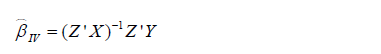
Direct IV analysis can be performed with the following R code:

Two-stage least square (2SLS) method is commonly used for IV analysis (9), which involves two stages. The first stage regress X on Z: . The estimated coefficients 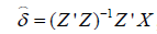 , and the predicted value is estimated as:

The second stage is to regress Y on the predicted values from the first stage: 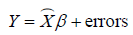 . The estimated 2SLS coefficient can be computed as:
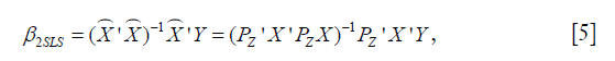
Note that PZ is a symmetric and idempotent matrix that PZPZ' =PZPZ = PZ. Equation [5] can be written as:

In the artificial example, X = [age, percent] and Z = [stage, age]. Recall that confounders other than the IV should be included in the first stage model on treatment in addition to the IV, so the covariate age was included in the vector Z in the first stage model. The 2SLS estimation can be performed using the following R code:

The solve() function is used to solve an equation a %*% x = b for x, where b can be either a vector or a matrix. The inverse of a matrix is to solve an equation with b = identity matrix. In the solve() function, b is taken to be an identity matrix by default (e.g., b argument is missing), which is the case in the above example. The result shows that the coefficient for percent is −39.7, which approximates the true effect size of −36.6. In case the number of instruments is equal to the number of endogenous predictors (e.g., an endogenous variable is correlated with both the independent variable in the model, and with the error term), direct IV estimation is equivalent to the 2SLS method (the model is just identified).
Analysis with ivreg() function
IV analysis with continuous outcome can be easily performed using the ivreg() function in the AER package (version 1.2-5) (10).

The ivreg() function fits IV regression by using 2SLS, which is equivalent to direct IV estimation when the number of instruments is equal to the number of predictors. The first argument specifies a formula with the regression relationship and the instruments. The formula has three parts in the form of y ~ x1 + x2 | z1 + z2 + z3, where y is the outcome variable, xs are endogenous variables and zs are instruments. Exogenous variables (e.g., a variable which is unaffected by other variables within an model) such as “age” in our example should be included in both sides of “|” symbol. The returned values can be extracted with the summary() function. Diagnostics of the model is returned by setting diagnostics = TRUE.

The results show that the coefficient for the variable percent is −39.7, which is exactly the same with that obtained by manual calculation.

The diagnostic statistics of IV analysis are shown in the above output. The strength of the IV can be evaluated with the partial first-stage F statistic. An IV is considered as a weak IV if the partial F statistic is less than 10 in the first stage model, that is, its impact on the choice of treatment is weak. A weak IV could lead to a larger variance in the coefficient, and severe finite-sample bias (11). The partial first-stage F statistic of 8056 indicates that stage is a strong IV in the study. Durbin-Wu-Hausman test compares the ordinary least square (OLS) estimate versus the IV estimate of the treatment effect assuming homogeneous treatment effects, that is, the treatment effect is the same at different levels of covariates (12,13). The rejection of the null hypothesis can be due to unmeasured confounding or heterogeneous treatment effects. Alternatively, Guo et al. [2014] proposed a test with an IV for unmeasured confounding, which distinguishes from treatment effect heterogeneity (14). There was no evidence of unmeasured confounding in the EN feeding study (P<0.001 for Durbin-Wu-Hausman test). Sargan is a test of instrument exogeneity using overidentifying restrictions, called the J-statistic in Stock and Watson. In case when there are more instruments than endogenous variables, the model is overidentified, and we have some excess information. To have consistent treatment estimates, all the IV should be valid. The test examines if all the IVs are in fact exogenous, that is, uncorrelated with the model residuals. The rejection of the null hypothesis of this global test indicates that at least one IV is invalid (15). Sargan test works when there are more IVs than endogenous variables, thus it is not applicable in our example.
Logistic regression for binary outcome
In case when the outcome variable is binary, IV analysis can be performed by fitting generalized model to the binary outcome. Probit and Logistic regression models are most commonly used (16). In this section, we will introduce the logistic regression model approach and probit model will be introduced in the next section. In analogy with the 2SLS method, two-stage predictor substitution (2SPS) method can be applied when the outcome is a binary variable (17). 2SPS works by first regressing the treatment X on the IV Z and observed exogenous covariates Xe, obtaining predicted and then fit a logistic regression of Y on and Xe. R code for performing the procedure is as follows:

The first line regresses variable “percent on stage” (Z) and “age” (exogenous covariate Xe). Then the predict function is employed to estimate the predicted percent (). In the second stage, the binary variable “mort” is regressed on the predicted “percent” and “age” in a logistic model. By default, the logit link function is used for binomial distribution outcome.

The variable “phat” in the above table is the predicted value of “percent” by the model s1. The results show that the coefficient of percent is −0.97, which is consistent with the true value of −0.97. However, this method is biased due to the non-collapsibility of the logistic regression (18).
Alternatively, the two-stage residual inclusion (2SRI) method can be used to estimate the true effect of an endogenous treatment. The first stage is the same as that in 2SPS. The second stage fits a logistic regression model for Y on Xe, X and the residual from the first stage. The estimated coefficient for X in second stage is the estimate of treatment effect.

The residual of the first stage linear regression is obtained using the residuals.lm() function. The results show that the effect of treatment deviates a little from the true effect (−0.99 vs. −0.97), but is much better than the naïve logistic regression model (−1.22). Similar to 2SPS, 2SRI has been shown to be asymptotically biased except when there is no unmeasured confounding (18).
Control function approach for binary outcome
Blundell and Powell proposed a control function approach to deal with endogeneity (19). Similar to the 2SRI method, the first step of the control function approach regresses treatment X on the IV Z and observed exogenous covariates Xe, then collects the residuals  . The second step estimates the probit model of interest, by including the first stage residuals as an additional regressor. This method is termed the control function approach, as the inclusion of controls for the correlation between v and ε, where ε is the structural error term in the Y = Xβ + ε equation.
Average structural function (ASF) is the probability of response variable given values of regressors, in the absence of endogeneity.

Where  is the mean of a vector of covariates including the treatment variable,
  is the estimated coefficient in the second stage, is the estimated coefficient for in the second stage. is the residual obtained from the first stage for each patient (i). Φ() is a function that transforms the linear predictor into probability scale. Then, ASF is the average of predicted probability. In the example, the treatment variable is allowed to vary across a range so that its effect on the probability of response variable can be shown. Suppose the variable “sofa” is known, then the true ASF can be obtained.

The above code holds covariates at their mean values and the treatment variable “percent” is allowed to vary between maximum and minimum values. A total of 50 values were generated. The coefficients used for data generating are used here to compute linear predictor (lprd). The linear predictor is then transformed into probability with logit transformation. Suppose the “sofa” is not known in the study, and we perform naïve probit regression model. The estimated ASF can be obtained with the following code.

The above computation is the same as the estimation of the true ASF, except that the variable “sofa” is unknown. The “percent” varies in the same range.
Then we proceed to estimate treatment effect with the two-step control function approach.

The two-stage control function approach is similar to 2SRI method except that the residual is scaled in the example. The following code is to estimate ASF:

The for() function is used to loop through all 50 values of percent. Within each loop, there is 1,000 v1 values and thus 1,000 predicted response values. We need to take the mean of these response values to obtain the mean probability for each given value of “percent”.

Figure 2 plots the probability of mortality against “percent”. The result showed that while the two-step probit model is consistent with the true model, the naïve probit model is biased. Also note the three lines are straight, which is attributable to the range of percent is restricted between 0 and 1. If the range of percent is extended, between −10 and 10, for example, the shape of these curves will be sigmoid.

Local average response function (LARF)
Theoretical basis of the LARF method was developed by Abadie (20). The method involves two steps: the first step constructs pseudo-weights according to the probability of receiving the treatment instrument; and the second step involves the computation of LARF conditional on covariates and treatment by using pseudo-weights. Mathematical details of the LARF is not reviewed here and readers can consult the references (20,21). In this section, we focus on how to implement the LARF method to estimate treatment effect in the presence of endogeneity. The LARF package (version: 1.4) is employed for this purpose (21).

The result is not as expected. The value −75.2 is the estimate consistent with the naïve biased estimate. Since the LARF requires treatment variable to be binary, we simulate the sample in another way.

The use of LARF method appears to adjust some of the biases induced by ignoring a confounding factor sofa. The true effect is −40.5, the naïve biased estimate is −59.9, and the LARF result is −45.3. The result is reasonable for continuous outcome cost.trt. However, it is not the case for binary outcome mort.trt.

The results of LARF method seems to bias the effect size more than the naïve regression model. Possibly, estimation with one random dataset may cause bias and simulation with 1000 or more times may be necessary in order to obtain the true estimates.
Discussion
In this article, we discussed some methods for IV analysis and showed R code for the performance of them. The manual analysis is complex and requires some knowledges on matrix manipulation. This is not suitable for research practice but can help to understand how IV analysis works. 2SLS method is commonly used for IV analysis. It is a natural starting point of IV analysis, and the estimate is asymptotically unbiased. However, 2SLS estimate can be biased in binary cases or in the case of non-linear models. 2SPS can be applied when the outcome is a binary variable. However, 2SPS in non-linear model does not always yield consistent exposure effects on the outcome, and parameter estimation process is more difficult than 2SLS. 2SPS may not provide causal OR under a logistic regression model. 2SRI is able to yield consistent estimates for both linear and non-linear models. It performs better than 2SPS. 2SPS is suitable in the case of a binary exposure with a binary or count outcome. LARF is suitable for estimating treatment effect when both the treatment and its instrument are binary.
Acknowledgements
Funding: This study was supported by funding from Zhejiang Provincial Natural Science Foundation of China (LGF18H150005) to Z Zhang.
Footnote
Conflicts of Interest: The authors have no conflicts of interest to declare.
References
- Grobbee DE, Hoes AW. Clinical Epidemiology: Principles, Methods, And Applications For Clinical Research. 1st edition. Jones & Bartlett Learning, 2008.
- Klungel OH, Martens EP, Psaty BM, et al. Methods to assess intended effects of drug treatment in observational studies are reviewed. J Clin Epidemiol 2004;57:1223-31. [Crossref] [PubMed]
- Angrist JD, Imbens GW. Identification and Estimation of Local Average Treatment Effects. Cambridge, MA: National Bureau of Economic Research, 1995.
- Uddin MJ, Groenwold RH, Ali MS, et al. Methods to control for unmeasured confounding in pharmacoepidemiology: an overview. Int J Clin Pharm 2016;38:714-23. [PubMed]
- Klungel OH, Jamal Uddin M, de Boer A, et al. Instrumental Variable Analysis in Epidemiologic Studies: An Overview of the Estimation Methods. Pharm Anal Acta 2015;6:353.
- Zhang Z, Li Q, Jiang L, et al. Effectiveness of enteral feeding protocol on clinical outcomes in critically ill patients: a study protocol for before-and-after design. Ann Transl Med 2016;4:308-8. [Crossref] [PubMed]
- Li Q, Zhang Z, Xie B, et al. Effectiveness of enteral feeding protocol on clinical outcomes in critically ill patients: A before and after study. PLoS One 2017;12:e0182393. [Crossref] [PubMed]
- Baiocchi M, Cheng J, Small DS. Instrumental variable methods for causal inference. Stat Med 2014;33:2297-340. [Crossref] [PubMed]
- James LR, Singh BK. An introduction to the logic, assumptions, and basic analytic procedures of two-stage least squares. Psychol Bull 1978;85:1104-22. [Crossref]
- Kleiber C, Zeileis A. Applied Econometrics with R. Springer, 2008.
- Stock JH, Wright JH, Yogo M. A survey of weak instruments and weak identification in generalized method of moments. J Bus Econ Stat 2002;20:518-29. [Crossref]
- Wu DM. Alternative Tests of Independence between Stochastic Regressors and Disturbances: Finite Sample Results. Econometrica 1974;42:529-46. [Crossref]
- Hausman JA. Specification Tests in Econometrics. Econometrica 1978;46:1251-71. [Crossref]
- Guo Z, Cheng J, Lorch SA, et al. Using an instrumental variable to test for unmeasured confounding. Stat Med 2014;33:3528-46. [Crossref] [PubMed]
- Small DS. Sensitivity Analysis for Instrumental Variables Regression With Overidentifying Restrictions. J Am Stat Assoc 2007;102:1049-58. [Crossref]
- Clarke PS, Windmeijer F. Instrumental Variable Estimators for Binary Outcomes. J Am Stat Assoc 2012;107:1638-52. [Crossref]
- Terza JV, Basu A, Rathouz PJ. Two-stage residual inclusion estimation: addressing endogeneity in health econometric modeling. J Health Econ 2008;27:531-43. [Crossref] [PubMed]
- Cai B, Small DS, Have TR. Two-stage instrumental variable methods for estimating the causal odds ratio: analysis of bias. Stat Med 2011;30:1809-24. [Crossref] [PubMed]
- Blundell RW, Powell JL. Endogeneity in Semiparametric Binary Response Models. Rev Econ Stud 2014;71:655-79. [Crossref]
- Abadie A. Semiparametric instrumental variable estimation of treatment response models. J Econom 2003;113:231-63. [Crossref]
- An W, Wang X. LARF: Instrumental Variable Estimation of Causal Effects through Local Average Response Functions. J Stat Softw 2016;71:1-13. [Crossref]

