

Reinforcement learning in clinical medicine: a method to optimize dynamic treatment regime over time
Introduction
Precision medicine is an important concept in the modern era, which dictates that the treatment regime should be individualized depending on genetic background, demographics and clinical characteristics. Many clinical conditions can be extremely heterogeneous that the treatment regime is highly variable. For example, sepsis is a heterogeneous syndrome which is characterized by different clinical outcomes and responses to fluid resuscitation (1). Treatment regimes should be individualized for different subphenotypes. Even for a certain subphenotype, the treatment regime can evolve over time. Thus, individualized dynamic treatment regime should be adopted to achieve the best potential outcome. Reinforcement learning (RL) is a powerful method in computer science that has been successfully used to teach an agent to learn to interact with the environment, aiming to achieve the best reward/return. This is quite similar to the situation in clinical practice, where a doctor needs to adopt an action (treatment regime) depending on a patient’s conditions (e.g., demographics, genetic background, clinical characteristics and previous response to a specific treatment regime). Thus, reinforcement learning can be used to solve a clinical decision problem, whereby the concept of precision medicine can be realized. In this review article, we will introduce (I) the concept of reinforcement learning, (II) how this concept can be adopted to clinical research, and (III) how to perform RL using R language.
Basic ideas behind reinforcement learning
The key elements of a RL system include a policy, a reward signal, a value function and a model of the environment (Figure 1). A policy is usually a function mapping from a state to an action. A policy defines how an agent takes action in response to the environment. A reward defines the goal of a RL problem. Every time (t) when an agent takes an action (at) on the environment, the environment sends a reward signal (rt+1) to the agent. The goal of the agent is to maximize the reward by taking an appropriate action. While the reward signal indicates the immediate benefit after taking an action, the value function defines the long-term benefit. The value of a state is the total amount of reward an agent can expect to accumulate over time, starting from that state. For example, when a doctor resuscitates a patient with septic shock, the action space comprises vasoactive agents and fluid infusion, and the immediate reward can be a stabilized blood pressure, or a normalized serum lactate (2). Since the policy is a mapping from the state to an action, the doctor will make treatment decision depending on the environment state of the patient. The mortality outcome at hospital discharge can be considered as a final reward. The state space of septic shock can be any combinations of hemodynamics, electrolytes, serum lactate and demographics. However, this can be an extremely large space due to the curse of dimensionality, and dimension reduction is usually required (3).

However, several key assumptions that are commonly used in RL in computer science may not be applicable in clinical trials. First, many RL algorithms such as dynamic programming requires that the complete knowledge of the environment is known (based on physical laws and domain knowledges), which however is usually unsatisfied in clinical data. In the septic shock example, the underlying mechanisms behind hospital mortality cannot be represented by a deterministic equation and must be estimated from samples. Second, the data collection can be cheap and easy to perform in some RL examples such as the blackjack, in which tens of thousands of episodes of the game can be simulated (i.e., the data generating mechanism is known). This is not true in clinical setting because the sample size is usually limited and collecting data is expensive (e.g., also for the confidential issues). Of note, the state space and action space can be larger than the sample size in most situations, and thus parametric models are usually required to model the data. Third, the Markov property is assumed to be true in computer science, which is defined that the probability of each possible value for St and Rt depends only on the immediately preceding state (St−1) and action (At−1), but not on earlier states and actions. However, there is no such assumption from the pathophysiology that earlier conditions have no causal association with final clinical outcome. Thus, the notion of history must be introduced in solving clinical problems. The history at a given stage includes all the present and past states, plus the present action. As a result, the history space grows exponentially with the number of stages (4).
Working example
A simulated dataset is created for the illustration purpose.

As noted above, a data frame is generated with two stages. On stage 1, there are three covariates denoted as x11, x12 and x13; and treatment was A1. On stage 2, the three covariates are x21, x22 and x23, and the treatment is A2. Finally, we observe an outcome which is a continuous variable. Higher values indicate a better outcome. For stage 1, the optimal decision rule dictates that A1 should take value 1 for subjects with x11 >-0.54 and x12 <0.54. However, clinicians choose A1 value by a logit function (the propensity function) in clinical practice. Thus, the A1 used in real world practice may not equal the value adopted by the optimal rule. The purpose of RL is to learn the optimal rule to maximize the outcome Y. In the same vein, the optimal decision rule for A2 is to assign A2=1 to subjects with x21 >0.3 and x23 <0.46. However, the exact form of the outcome function is not easy to specify but can be approximated.
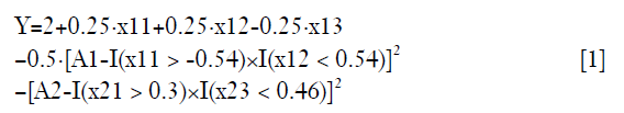
There is an indicator function I(·) which returns 1 when the express is true, and 0 otherwise. The quadratic function suggests that the outcome Y can only be maximized when A1 and A2 is equal to the value determined by the optimal decision rule in both stage 1 and 2.
Q-learning algorithm
Q-learning is a temporal difference control algorithm that can be used to estimate optimal dynamic treatment regime from longitudinal clinical data. Suppose there are two stages, the Q function can be defined as (5):
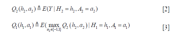
The Q function at t=2 measures is the value function of assigning  to a patient with history
  . In a similar sense, the Q function at t=1 measures the quality of assigning
  to a patient with history
  , assuming an optimal regime at stage 2 is adopted. The first step of Q learning is the regress Y on H1 and A2 to obtain estimators of
  :
:
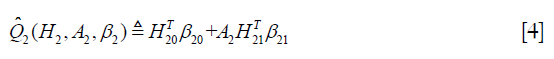
Where H2 includes history variables up to t=2; H20 is the main effect model (treatment-free) consisting a subset of variables in H2. Similarly, H21 is also a subset of variables of H2 for the contrast function. A contrast function defines how the expected outcome varies depending on treatment regime. The only means by which the treatment can influence outcome are via the contrast function (6).
The second step is to maximize the Q2 function by varying A2. In the above example, if A2 takes value {-1, 1}, we can define 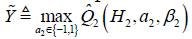 , which gives
 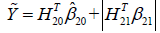 .
.  is the potential outcome when optimal regime is adopted at stage 2. Finally, the estimated is regressed on H1 and A2 to obtain
  in the model

The optimal regime at stage one can be obtained by maximizing the above equation.
Q-learning with R
In the example, the DynTxRegime package (v4.1) will be used to obtain optimal regime at each stage. The package iqLearn is also available in R that performs Q-learning algorithm (5).

The above code creates two components (e.g. the main effect and the contrast components) of the outcome model. Note that all covariates are specified to be predictive on the outcome, and only covariates collected at stage two determine the optimal decision rule. However, the functional form is mis-specified in the above equation.

The second stage can be fit by using the above code. We can create a confusion matrix to see whether the learning algorithm can assign optimal regime to more subjects in the training set, than that assigned by the physician (e.g., suppose the longitudinal data were collected from electronic healthcare records and the treatment was determined by physicians).

The result shows that the Q-learning method is not able to assign optimal regime to more subjects than that assigned by physicians. In the observational cohort (the first matrix), 217 patients received A2=0, and 71 received A2=1, which are optimal regimes. The Q-learning algorithm correctly assigned A2=0 to 357 patients, and A2=1 to 71 patients. Other patients fail to receive the optimal regime if treatment regime is determined by the Q-learning algorithm. This is due to the misspecification of the outcome linear function, which has been widely discussed in the literature (7,8).
Q-learning is implemented through a backward recursive fitting procedure based on a dynamic programming algorithm. The previous step fitted a linear regression model for stage two, and next we will regress the estimated outcome on covariates (X1) and treatment (A1) at stage one.

The specification of the regression model is similar to that at for stage two except that the response argument takes an object returned by previous fit. The coefficient for the first stage model can be examined by the following code:

Again, the confusion matrix can help to examine the correctness of Q-learning algorithm to assign optimal regime.

It appears that the Q-learning algorithm fails to assign optimal regime to more subjects than the physicians’ judgement. However, the linear model cannot correctly capture the function form as that for data generation.
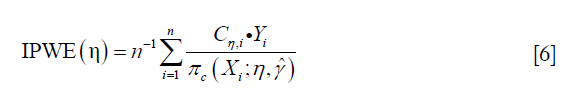
Inverse probability weighted estimator (IPWE)
To circumvent the risk of model misspecification as demonstrated above, the inverse probability weighted estimator for the population mean outcome can be employed (9). The estimator for E{Y*(gη)} is:
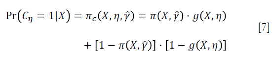
Where Cη=A·g(X,η)+(1−A)·[1−g(X,η)], and g(X,η)∈Gη is a specific treatment regime conditional on covariate X and coefficient η. The equation indicates that the observed outcome Y (under treatment A) is the counterfactual outcome Y*(gη) (under treatment g(X,η)) when Cη=1. Otherwise, Y*(gη) is not observed because a patient actually received treatment A is not equal to g(X,η). Suppose the treatment regime can only takes value 0 or 1. 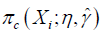 is the probability of Cη=1 giving covariates X:
The estimator IPWE(η) is actually a weighted average of observed outcome under decision rule g(X,η). Observed outcome Y not following the decision rule was excluded (by the Cη,i factor in the numerator) from the calculation. For patients who actually receive A=0, by substituting A=0 into the IPWE(η) equation, the contrast function can be written as:
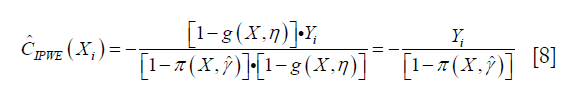
Similarly, the contrast function for A=1 can be written as:
Collectively, the contrast function is written as:
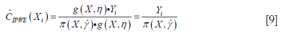
From the above discussion, we note that only the propensity model is required in the estimation, the mean outcome model is not required, which reduces the risk of model misspecification. We then define a function Z=I(C(X)>0), so that Z=1 indicate subjects who will benefit from treatment A=1 than A=0. The optimization problem can be regarded as minimization of a weighted misclassification error:
Where  is an estimate of contrast function for each subject. The problem can be considered as a classification problem with
  as the binary response, Xi as the predictor and
  as the weight. Classification and regression trees (CART) can be used to solve this problem (10).
The following code builds a propensity score model in which the variables x21 and x22 determine the choice of treatment regime. Since treatment A is a binary variable, a generalized linear model with the response variable following binomial distribution.

Then, the rpart package (version 4.1-13) is employed to solve the classification problem. The CART model uses x21, x22 and x23 as the predictors.

The second-stage analysis using IPW can be done with the following code.

Recall that the optimal decision rule is to assign A=1 to subjects with x21 >0.3 and x23 <0.46. The CART assigns x21 ≥0.15 and x23 <0.49 to receive A=1; but there are still moderate misclassifications (Figure 2).

The confusion matrix can be obtained with the following code.

The results showed that the IPW method can significantly improve the accuracy of assigning optimal regime to patients. There are only 50 patients who would benefit from A=0 but receive A=1 as determined by the IPW method.
Augmented Inverse Probability Weighted Estimators (AIPWE)
The IPWE method does not depend on parametric or semi-parametric at all, making it robust to model misspecification. However, the IPWE estimator of contrast values can be too noisy to successfully inform the classification regime. One method to circumvent the problem is to maximize on a doubly robust augmented inverse probability weighted estimator (AIPWE) for the population mean outcome over all possible regimes (9,11). The AIPWE for the mean outcome is given by:
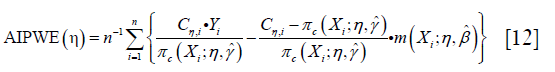
The m(Xi;η,β)=μ(1,X,β)·g(X,η)+μ(0,X,β)·[1-g(X,η)] is a model for the potential outcome under treatment regime gη that E(Y*(gη)|X)=μ(1,X)·g(X,η)+μ(0,X)·[1−g(X,η)]. AIPWE possesses the doubly robust property that the estimate is consistent for E(Y*(gη)) if either π(X,γ) or μ(A,X,β) is correctly specified. The contrast function for AIPWE estimator can be derived from the equation:
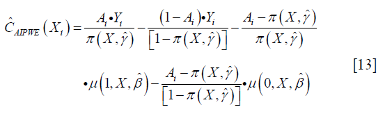
The only difference between  and
and  is that the former borrows information from specified parametric regression model of outcome μ(A,X,β), trying to strike a balance between two extremes that are non-parametric or completely depending on the parametric model (11). R code to perform AIPWE is very similar to that for IPWE, but we need to define the parametric outcome model. The outcome model is defined as

then the second stage for AIPWE analysis is:

Note that the only difference between AIPWE and IPWE is the use of parametric outcome model as specified by the moMain and moCont arguments. We know from the Q-learning section that the linear outcome model is mis-specified. The confusion matrix is examined in the following code:

The results show that the AIPWE significantly improve the accuracy of correctly assigning optimal regime to the patients. In this analysis, only 18 subjects are incorrectly assigned A=1 by the AIPW method, and 15 subjects are falsely assigned A=0. This number is better than the IPWE method.

The decision tree shows that x21 and x23 are used to split most nodes (Figure 3). Subjects with x21 <0.3 were correctly assigned A=0. The subjects with x23 ≥0.46 are also correctly assigned to receive A=0.

The first stage decision rule can be learned in a recursive manner as that for stage two. The only difference is that the predictors for both outcome model and propensity model are chosen from x11, x12 and x13. Furthermore, the response argument in the optimalClass() function receives the object returned in the stage two analysis.
Firstly, we define the propensity for treatment model and methods. Here the variable x11 and x12 are used to predict treatment assignment.

Secondly, we define the classification model in which the CART method is used. Other machine learning methods such as support vector machine are also allowed and can be passed to the buildModelObj() function by the solver.method argument.

Thirdly, we define the outcome model which is composed of the main effect model and contrast model.

Finally, the AIPWE model can be fit with the optimalClass() as before. Note that an optimalClass object is assigned to the response argument, which passes the counterfactual outcome under optimal treatment at stage two to the modeling strategy for the first stage. This is consistent with the idea behind reinforcement learning algorithm in computer science that the action-value function is updated by assuming all subsequent steps takes the optimal action to maximize the action-value function.

The data generating mechanism dictates that optimal regime A=1 should be given to subjects with x11 > −0.54 and x12 <0.54. The majority of subjects receiving A=1 following the AIPWE rule is those with x11 >−0.52, x12 <0.57 and x12 >−1 (Figure 4). Classification accuracy can be further examined with confusion matrix:


The above output shows that the treatment options made by physician misclassify 95 subjects to the A=1 and 140 to the A=0 group. The AIPWE rule is able to significantly improve the classification accuracy. Only 19 subjects are misclassified to A=1 group and 30 subjects are misclassified to the A=0 group.
Final remarks
Exploring dynamic treatment regime borrows ideas from the reinforcement learning algorithm from the computer science. The Q-learning algorithm is easy to interpret for domain experts, but it is limited by the risk of misspecification of the linear outcome model. IPWE overcomes this problem by non-parametric modeling that the mean outcome is estimated by weighting the observed outcome. AIPWE borrows information from both the propensity model and mean outcome model and enjoys the property of double robustness. However, these statistical method does not allow the action space to have multiple levels. In real clinical practice, the interest may focus on the combinations of treatment regime, giving rise to a multi-dimensional action space.
Acknowledgments
None.
Footnote
Conflicts of Interest: The author has no conflicts of interest to declare.
Ethical Statement: The author is accountable for all aspects of the work in ensuring that questions related to the accuracy or integrity of any part of the work are appropriately investigated and resolved.
References
- Zhang Z, Zhang G, Goyal H, et al. Identification of subclasses of sepsis that showed different clinical outcomes and responses to amount of fluid resuscitation: a latent profile analysis. Crit Care 2018;22:347. [Crossref] [PubMed]
- Raghu A, Komorowski M, Ahmed I, et al. Deep Reinforcement Learning for Sepsis Treatment. Vol. cs.AI, arXiv.org. 2017.
- Komorowski M, Celi LA, Badawi O, et al. The Artificial Intelligence Clinician learns optimal treatment strategies for sepsis in intensive care. Nat Med 2018;24:1716-20. [Crossref] [PubMed]
- Statistical Methods for Dynamic Treatment Regimes - Reinforcement Learning, Causal Inference, and Personalized Medicine | Bibhas Chakraborty | Springer. New York: Springer-Verlag, 2013 Jan 1. Available online: https://www.springer.com/us/book/9781461474272
- Linn KA, Laber EB, Stefanski LA. iqLearn: Interactive Q-Learning in R. J Stat Softw 2015.64. [PubMed]
- Wallace MP, Moodie EE, Stephens DA. Dynamic Treatment Regimen Estimation via Regression-Based Techniques: Introducing R Package DTRreg. Journal of Statistical Software 2017;80. [Crossref]
- Wallace MP, Moodie EE. Doubly-robust dynamic treatment regimen estimation via weighted least squares. Biometrics 2015;71:636-44. [Crossref] [PubMed]
- Barrett JK, Henderson R, Rosthøj S. Doubly Robust Estimation of Optimal Dynamic Treatment Regimes. Stat Biosci 2014;6:244-60. [Crossref] [PubMed]
- Zhang B, Tsiatis AA, Laber EB, et al. A robust method for estimating optimal treatment regimes. Biometrics 2012;68:1010-8. [Crossref] [PubMed]
- Loh WY. Classification and regression trees. Wiley Interdisciplinary Reviews: Data Mining and Knowledge Discovery 2011;1:14-23. [Crossref]
- Zhang B, Tsiatis AA, Davidian M, et al. Estimating Optimal Treatment Regimes from a Classification Perspective. Stat 2012;1:103-14. [Crossref] [PubMed]

