
Drawing Nomograms with R: applications to categorical outcome and survival data
Introduction
The definition of nomogram is well described in Wikipedia that “A nomogram (from Greek νόμος nomos, “law” and γραμμή grammē, “line”), also called a nomograph, alignment chart or abaque, is a graphical calculating device, a two-dimensional diagram designed to allow the approximate graphical computation of a mathematical function.” A nomogram consists of a set of scales that each scale represents a characteristic of study population. If there are interaction terms in the original regression model, there will several scales representing certain combinations of interacting variables. Nomogram is actually a visualization of a complex model equation that the behavior of a predictor is represented in scales (1). In clinical medicine, the tool is widely used for prediction of patients’ outcomes, considering his or her clinical characteristics. Nomogram is most widely used in clinical oncology to help patients and doctors to make important treatment decisions (2).
Because nomogram is based on regression models such as logistic regression model, parametric survival model and ordinal logistic regression model, the performance of the tool is dependent on the regression models. The discrimination, calibration, and external validation also apply to the nomogram. Therefore, model diagnostics and model fit that are applicable to regression models should also be performed before drawing a nomogram. In this article, these tasks are not described, but readers can consult other tutorials of the big-data clinical trial column (3,4). This article focuses on how to draw a nomogram with R software and how to adjust some interesting and important parameters.
Worked example
The worked example and model strategies for drawing nomograms are adapted from the R documentation. In the following code, a data frame containing 1,000 observations and 6 variables are created. The variable age follows a normal distribution with a mean of 65 and standard deviation of 11. Lactate (lac) also follows a normal distribution, but abs() function is employed to ensure positive values. Sex and shock are generated as a factor variable. Arbitrary coefficients are given to each variable to produce a linear combination. plogis() function is called the ‘inverse logit’ that it gives probability according to the linear predictor.

Next, an ordinal categorical variable Y is created. The ifelse() function is useful to create categorical variable. All vectors are combined to create a data frame. Variable names and labels can be used to annotate nomogram, depending on the preference of the investigator. Often, the variable name is usually simple with abbreviations, and the label gives more details on the variable. Therefore, annotation with names makes the nomogram simple, whereas variable labels make the plot more informative. Both methods are illustrated in our example. Here, we assign labels to each variable.

Nomogram for binary outcome
Binary outcome is the most commonly encountered data type in clinical medicine, and can be modeled with logistic regression model. The outcome of interest for prediction is the probability of the event of interest, because this quantity is more intuitive for both clinicians and patients. In the example below, we labeled the outcome as “Risk of death”, which is a patient-important outcome variable.

In the article, the rms package is employed to fit regression model and depict nomogram. The rms package contains a collection of functions assisting model building and visualization. In essence, nomogram is a kind of visualization of regression models. Firstly, we need to define the distribution summaries for predictor variable with the datadist() function. Specifically, datadist() defines summary statistics for continuous and categorical predictors. These summary statistics include effect and plotting ranges, values to adjust to, and overall ranges. Nomogram only uses the list of categories from datadist() for categorical variables, and the outer limits for continuous ones. The object returned by datadist() is then assigned to option() function that later predictions and summaries of the fit will not need to access the original data used in the fit. Model fit is performed by lrm() function which is designed to fit logistic regression model. The nomogram() function first takes an object returned by regression model fit. In the example, it is the object name mod. The argument lp.at takes a vector of numeric values ranging from −3 to 4 by a step of 0.5. These values will be displayed in the linear predictor axis. A linear predictor function is a linear function (linear combination) of a set of coefficients and explanatory variables (independent variables), whose value is used to predict the outcome of a variable. The argument fun is optimal that it defines the transformation of linear predictor and plots it on another axis. In the example, the inverse-logit transformation is employed to transform linear predictor to the probability. Labels of function axis are defined by a vector of numeric values with fun.at argument. In the example, the linear predictor −3 is the minimum value and it corresponds to probability of 0.0474, thus only function values greater than 0.0474 can be displayed on function axis. In other words, the initial two values 0.001 and 0.01 will be omitted in nomogram. The funlabel argument is to change the name of function axis to “Risk of Death”. The conf.int argument gives confidence interval to display for each score. The default is to display no confidence limits. In the example, we want to display 0.1 and 0.7 confidence intervals for each score. The narrow interval of 0.1 is useful to determine which score it corresponds to. The abbrev is set to true to abbreviate levels of categorical factors. However, it only abbreviates the factor variables of interaction terms in the current version, which is not consistent with the R documentation. When we set minlength=1, it actually uses minlength=4 for interaction terms. Tick marks for categorical predictors (the variable shock) are supposed to be abbreviated to letters of the alphabet, but actually it doesn’t.

The nomogram can be plotted with the generic plot() function (Figure 1). It takes an object of class “nomogram” that contains information used in plotting the axes. The lplabel argument is used to rename the linear predictor axis. If tick marks of function axis are too crowded and overlap with each other, one may specify the fun.side argument with a vector of numeric values 1 and 3. The numeral 1 is to position tick marks below axis and numeral 3 for above the axis. Note that the first element of fun.side corresponds to the first value in the vector defined by fun.at, rather than the first value displayed in the axis. Because the first two function values are omitted, the fun.side argument takes effect from the third element. The argument col.conf=c(‘red’,‘green’) specifies that the 0.1 confidence interval is draw with red color and the 0.7 confidence interval is drawn with green color. Confidence bars defined by the conf.int argument are drawn in the space between predictor axis, and the vertical range within which to draw confidence bars can be modified using the conf.space argument. The conf.space argument takes a two-element vector defining the beginning and ending of vertical range to draw confidence bars. In the example, we draw the first bar at 0.1 and the last at 0.5 [e.g., The entire range between main axis is defined to be 1). The label.every=3 specifies to label every 3 tick marks. Vertical reference lines are drawn with col.grid = gray(c(0.8, 0.95)] argument. Any colors can be designated to the color grid.

If we use abbreviations to label tick marks, a legend should be added with gend.nomabbrev() argument. The x and y arguments tell the function where the legend should be placed. The predictor to which the legend relates is specified in which argument.
Nomogram for ordinal outcome variable
Ordinal logistic regression is a type of logistic regression that deals with dependent variables that are ordinal—that is, there are multiple response levels and they have a specific order, but no exact spacing between the levels. In the example, the variable Y contains four levels. Similarly to the binary logistic regression model, ordinal model can be fit with lrm() function. In the model, an interaction between sex and lac is included. Furthermore, the variable lac takes a linear tail-restricted cubic spline function by using rcs() function.

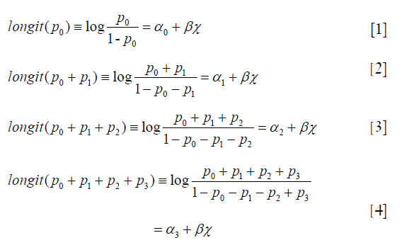
Here we will spend some time to discuss the estimated parameters from ordinal regression model. In the example, the outcome variable Y takes four levels (0, 1, 2 and 3), and the ordinal logistic regression model has the form:
Because p0+p1+p2+p3=1, the last Eq. [4] is not fit. This model is known as the proportional-odds model because the odds ratio (exponentiation of β) of the event is independent of the outcome category. The odds ratio is assumed to be constant for all categories. The model simultaneously estimated 3 equations and the comparisons of outcome categories are shown in Table 1. Eq. [1] models the odds of being in the set of Y=0 on the left versus the set of categories Y={1,2,3} on the right. Because ordinal regression assumes parallel regression, there is only one set of coefficients for each independent variable. Eqs. [1] to [3] share the same coefficient β for covariate x. However, the intercept would be different, as denoted by different annotations from α0 to α2. The intercepts can be used to calculate predicted probability for patients with given set of characteristics of being in a particular category (5).

Full table

The Newlabels() function is used to override the variable labels in a fit object. In the example, variable age is assigned a label named “Age in Years”. Parameters in the nomogram() function are similar to that in the above example.

The generic function plot() gives a nomogram for ordinal outcome variable (Figure 2). Since there is an interaction between sex and lac, continuous variable lac is depicted at two levels of sex. Note that there are three function axes. For each patient with given characteristics (e.g., the linear predictor is fixed), the probabilities of each category are different.

Nomogram for survival data
In follow up study, the time-to-event or survival data are commonly encountered. Multivariable analysis of such data includes semi-parametric and parametric regression modeling. Semi-parametric modeling provides the impact of covariates on survival time, but leaves baseline hazard function unspecified (6). On the other hand, parametric modeling assumes functional forms of the baseline hazard, by which a complete description of survival time can be performed (7). Interesting statistics in survival analysis include among others the survival probability at a given time point, and median survival time. If investigators are interested in several statistics for survival data, more than one transformation of the linear predictor would be plotted in nomogram.

To perform survival analysis, the survival package is employed. In this package, there is a data frame named lung containing variables of patients with advanced lung cancer from the North Central Cancer Treatment Group. Performance score (ph.ecog) rate how well the patient can perform usual daily activities (8). The variable sex is transformed to a factor, with labels male and female

Weibull survival model is fit with psm() function, which first takes an object of class Surv returned by Surv(). In the example, only three variables ph.ecog, sex and age are used. Weibull distribution of survival time is specified with the “dist=‘weibull’” argument. Other options include “exponential”, “gaussian”, “logistic”, “lognormal” and “loglogistic”.

The above two lines define two functions med and surv. The med() will take values of linear predictor and return median survival time. By default, the function returns median survival time, but survival time of other quantiles can be specified with q argument. The surv() function will take a time and linear predictor as arguments, and return the probability of survival to that time. R code to produce nomograms for survival data are as follows.

Figure 3 shows the nomogram for median and 1-Q survival time. For practical users, it is easy to refer a patient with given characteristics to the corresponding median and 1-Q survival time. In Figure 4, there are two function axes for 200- and 400-day survival probabilities.


Nomogram for semiparametric survival models
Semiparametric survival model, also known as the Cox proportional hazard model, is far more popular in medical literature. Thus, in this section we show how to fit a Cox proportional hazard model with R and draw a nomogram based on the Cox proportional hazard model. Again we use the lung dataset as the above example. The Cox proportional hazard model can be fit with cph() function in the rms package.

The result is shown in Figure 5. Of note, the linear predictor axis is omitted because most users don’t care about it. Other arguments of the nomogram() function and interpretation of results are similar to previous examples.

Acknowledgements
None.
Footnote
Conflicts of Interest: The authors have no conflicts of interest to declare.
References
- Kattan MW, Marasco J. What is a real nomogram? Semin Oncol 2010;37:23-6. [Crossref] [PubMed]
- Su D, Zhou X, Chen Q, et al. Prognostic Nomogram for Thoracic Esophageal Squamous Cell Carcinoma after Radical Esophagectomy. PLoS One 2015;10:e0124437. [Crossref] [PubMed]
- Zhang Z. Model building strategy for logistic regression: purposeful selection. Ann Transl Med 2016;4:111. [Crossref] [PubMed]
- Zhang Z. Residuals and regression diagnostics: focusing on logistic regression. Ann Transl Med 2016;4:195. [Crossref] [PubMed]
- Ordinal Logistic Regression. In: Harrell FE. Regression Modeling Strategies. New York, NY: Springer; 2001:331-43.
- Introduction to Survival Analysis. In: Harrell FE. Regression Modeling Strategies. New York, NY: Springer; 2001:389-412.
- Harrell FE. Parametric Survival Models. In: Regression Modeling Strategies. New York, NY: Springer; 2001:413-42.
- Loprinzi CL, Laurie JA, Wieand HS, et al. Prospective evaluation of prognostic variables from patient-completed questionnaires. North Central Cancer Treatment Group. J Clin Oncol 1994;12:601-7. [Crossref] [PubMed]

