Data management by using R: big data clinical research series
Introduction
Electronic medical record (EMR) system has already been widely used in most hospitals in China, and it can serve as a potential reservoir to provide resources for clinical research (1-3). EMR can be regarded as a form of big data because the data volume of EMR is ever expanding (4). All information of a patient, from outpatient medication to inpatient management, can be easily extracted from established database. Furthermore, hospital admissions and outpatient visits can be linked together by using unique patient identification number. However, clinicians are always experts in clinical practice but lack necessary skills in the management big data. They are usually overwhelmed by the complexity of the structure of EMR data. As a result, many research questions cannot be answered by using the readily available big data. To conduct a prospective experimental studies or observational studies is usually time consuming and even impossible for the extremely busy clinicians. To make ends meet, a series of articles introducing data management skills are put forward to guide clinicians to big data clinical research.
R
R is not a name of software, but it is a language and environment for data management, graphic plotting and statistical analysis (5,6). R is freely available and is an open source environment that is supported by world research community. Thousands of statistical and graphing packages are available for use, and the package pool is ever expanding. One attractive feature of R is its graphing capability, allowing for nearly any customizations of figures (7). R can be downloaded from Comprehensive R Archive Network (CRAN) at http://cran.r-project.org. Users can easily complete the installation following guidance on the website. After installation, R console should be launched where one can input commends for data analysis. In the following sections, I assume that users have already been familiar with the preparations of R. This section will focus on creating and recoding variables, renaming variable. Although these techniques look simple, they must be used in each project of big data exploration.
For the ease of reading, I denote codes that can be executed in R console with the beginning symbol “>”.
Working example
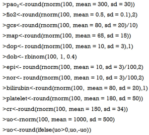
A data frame is created to include original variables such as PaO2, FiO2, Glasgow coma scale (GCS), mean arterial pressure (MAP), bilirubin, platelet count, creatinine and urine output. The simulated dataset was used for illustration purpose, and it has no practical meaning.
Continuous variables are created by assuming that they have a normal distribution, whereas categorical variables are created by assuming they have binomial distribution.
The function rnorm() is used to randomly generate variables with mean and standard deviation (sd) arguments. Because generated observations may have decimal places which is not in line with the real world situation, round() function was used to obtain integers (e.g., this function was applied to variable uo and GCS). Ifelse() function was used to convert negative variables into positive ones. rbinom() function is used to generate categorical variables with binomial distribution. In the calculation of SOFA score, we only need to know whether dobutamine is used or not. However, these steps generated separate vectors that are stored in R workplace and we need to combine them into a data frame.
The results are shown in Table 1. There are 100 observations in the dataset but only the first 8 are displayed. The first row is the variable name and the first column is the number of observations. This dataset illustrates a typical example that we can extract from EMR. We will use it for the illustration of several basic R functions in the following sections.

Full table
Creating new variable
It is common to create new variables in data analysis. These variables are called secondary variable, to distinguish them from original variable that can be extracted directly from EMR. In clinical practice, the most widely used secondary variable is varieties of scores. Particularly in critical care medicine, there are numerous risk stratification scores that can be calculated from original physiological and laboratory variables. Sequential Organ Failure Assessment (SOFA) score is one of such example and I would like to illustrate how it can be calculated from original variables.
SOFA score is used to determine the extent of organ functions. It is based on six different scores for respiratory, hepatic, cardiovascular, coagulation, neurological and renal systems (Table 2) (8). The SOFA score equals the sum of scores of each organ system, and it simplifies multi-dimension parameters into one dimension.

Full table
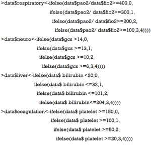
First, we calculate scores for each organ system. Because there are five categories for each system, we use the ifelse() function.
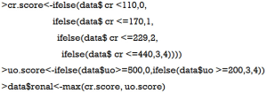
The renal score is a little more complex than others because it encompasses serum creatinine and urine output. The “or” relationship means that for an individual patient we used the maximum scores derived from either urine output or creatinine. Therefore, we first calculate scores for urine output or creatinine, respectively; then the maximum score was used as the final renal score.
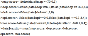
Scores for cardiovascular system comprises five variables (e.g., map, dop, dob, epi and nor). We can apply max() function with more variables as its arguments.
Then the total SOFA score can be calculated by summing all individual system scores.
We can now take a look at the new dataset by using head() function (Table 3). The dataset contains scores for each individual system (from variable cardio to coagulation) and the last column is the SOFA score.

Full table
Recoding variables
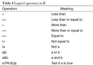
The most commonly used technique in recoding variable is to change a continuous variable into a set of categories. To recode data, one can use R’s logical operators (Table 4). These logical operators create logical expression and return the value of TRUE or FALSE.
Full table
Suppose that we want to make classifications of acute respiratory distress syndrome (ARDS) based on Berlin definition. This definition proposed 3 mutually exclusive categories of ARDS based on degree of hypoxemia: severe (PaO2/FiO2 ≤100 mmHg), moderate (100 mmHg < PaO2/FiO2 ≤200 mmHg), and mild (200 mmHg < PaO2/FiO2 ≤300 mmHg) (9). Then we can recode continuous variable PaO2/FiO2 to categorical variable berlin (severe, moderate and mild). First, we create a new variable named ‘oxyindex’.
Because patients with oxygen index greater than 500 are less likely to have ARDS, we need to exclude them.
This statement assigned null (NA) values to observations with oxygen index greater than 500. The statement ‘variable[conditions]<-expression’ takes value from expression when the condition is TRUE.
Next we can use the following code to create the berlin variable:
Data frame names are used in these codes to ensure the new variables are saved back to the data frame. Alternatively, if you do not want to repeat data frame name, you can use within() function to write the code more compactly.
Another very useful function shipped with R is cut(), which is able to convert continuous variable into factor variable.
The first argument of cut() function is a numeric vector to be converted to a factor variable. The second argument can be a numeric vector containing two or more cutoff points. The last argument labels each level of the factor variable. Note that we do not need to specify NA values to values greater than 500, and the newly created factor variable automatically excludes observations with oxygen index >500.
Renaming variables
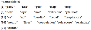
When working with big data, you may have hundreds of variables at hand and you need to rename variables to avoid confusion. In our example, if you are not happy with the name oxyindex, you can change it by using names() function.
As you can see, the names() function extract variable names of a data frame.
Alternatively, you can use rename() function for the same purpose (10). Rename() function is in the reshape package and you should load it to the working environment first.
This code looks more compact and it is particularly useful to change a series of variable names.
Summary
The educational article introduces some basic R functions for data management. Differently from other educational material, this article illustrates the R functions in the context of clinical research. The questions discussed were those that have been encountered by the author, and were considered as the most fundamental skills. Creating new variable is to create new variable based on other original variables that can be directly extracted from EMR. The ifelse() function is very useful. In recoding variables, logistical operators are always used. There is also a useful function called cut() which is able to convert continuous variable into factor variables. Renaming variable is applied when there are hundreds of variables and you are not satisfied with its original forms. The principle of naming variable is to make it concise and informative.
Acknowledgements
None.
Footnote
Conflicts of Interest: The author has no conflicts of interest to declare.
References
- Zhang Z. Big data and clinical research: focusing on the area of critical care medicine in mainland China. Quant Imaging Med Surg 2014;4:426-9. [PubMed]
- Zhang Z. Big data and clinical research: perspective from a clinician. J Thorac Dis 2014;6:1659-64. [PubMed]
- Monteith S, Glenn T, Geddes J, et al. Big data are coming to psychiatry: a general introduction. Int J Bipolar Disord 2015;3:21. [PubMed]
- Potash JB. Electronic medical records: fast track to big data in bipolar disorder. Am J Psychiatry 2015;172:310-1. [PubMed]
- Kabacoff R. R in Action. Shelter Island: Manning Publications Co., 2011.
- Lander JP. R for Everyone: Advanced Analytics and Graphics. Boston: Addison-Wesley Professional, 2014.
- Horton NJ, Kleinman K. Using R for data management, statistical analysis, and graphics. Clermont: CRC Press, 2010.
- Vincent JL, Moreno R, Takala J, et al. The SOFA (Sepsis-related Organ Failure Assessment) score to describe organ dysfunction/failure. Intensive Care Med 1996;22:707-10. [PubMed]
- ARDS Definition Task Force, Ranieri VM, Rubenfeld GD, et al. Acute respiratory distress syndrome: the Berlin Definition. JAMA 2012;307:2526-33. [PubMed]
- Wickham H. Reshaping data with the reshape package. Journal of Statistical Software 2007;21:1-20.


