

Statistical methods and models in the analysis of time to event data
Time to event data are common in medical research, where outcomes are the time until the occurrence of an event of interest that are subject to censoring. The main goal for the analysis of time to event data is to investigate the effects of covariates on the hazard for an event of interest and estimate the survival probability. The article by Zhou et al. (1) provides a nice overview on building a clinical prediction model on time to event data and assessing the prediction accuracy of a clinical prediction model, describing the model construction and model validation using R functions (1). The article introduces the Cox proportional hazards model (2) as a clinical prediction model for time to event data, which is the most widely used statistical model in studies of time to event data to estimate the effects of covariates on the hazard for an event of interest, and describes visualizing the survival probability for a patient with specific values of covariates using nomogram with R. The article also introduces R code to compute the concordance index (i.e., C-index) and draw a calibration plot to evaluate the discriminatory and calibration accuracy of a Cox regression model. However, the limitation of the article is that the authors did not describe about checking the proportional hazards assumption. In practice, the proportional hazards assumption may not be plausible for some applications. Thus, it is necessary to assess the proportionality assumption since a violation of the assumption may affect statistical inference. The most commonly used approaches for checking the assumption are to use a test based on the Schoenfeld residuals (3), and draw the Schoenfeld residuals plot (4) and the curves (5), where is the Kaplan-Meier estimator (6). A test based on the Schoenfeld residuals can be conducted using the function cox.zph() in survival package in R, which provides a two-sided P value for the test under the null hypothesis of proportionality. If a P value is less than the prespecified significance level, it indicates a violation of the proportionality assumption. The Schoenfeld residuals plot can be drawn using the function cox.zph() in R. When a covariate is continuous, if a plot of Schoenfeld residuals versus times for the covariate shows patterns other than a constant, it indicates that there is a departure from the proportionality assumption for the covariate. As another graphical check, a plot of versus log(time) can be used to investigate the assumption. If the curves for each of the levels of a covariate are parallel, it indicates that the proportional hazards assumption holds for the covariate. When the proportional hazards assumption does not hold for some covariates, other regression models may be used to estimate the effects of covariates on the hazard function for an event of interest. For example, an additive hazards model (7-9) or accelerated failure time model (10-12) can be used as alternatives to the proportional hazards model.
The clinical prediction model describes the relationship between covariates and outcomes of interest in forms of mathematical equations. However, in practice, it is often very hard to interpret the relationship between covariates and outcomes of interest and the effect of covariates intuitively. Several methods have been suggested to address the issue and a nomogram is one of the most widely used methods to visualize the model equations that present the behaviors of covariates in scale. Zhang and Kattan (13) describe how to create nomograms for a logistic regression model for categorical outcome and for a Cox regression model for survival outcome using R. Alternatively, presenting several scales for certain combinations of covariates of interest dynamically can be more helpful for practitioners to interpret the relationship between covariates and outcomes of interest and the effect of covariates. The DynNom package in R (14) provides DynNom function that creates a dynamic nomogram as shown in Figure 1, which uses the following example.

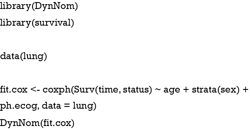
Using a dynamic nomogram, one can obtain the estimated survival probability with 95% confidence interval for a specific set of values of covariates dynamically and compare the magnitude of the effect of covariates on the hazard function interactively.
In medical research, it is crucial to develop an accurate model for prediction since it may be used in clinical decision making such as the choice of treatment options. This leads to evaluation of the prediction accuracy of a clinical prediction model. The prediction accuracy of a Cox regression model can be assessed by discrimination and calibration. The concordance index (C-index) and calibration plots have been widely used to evaluate the discriminatory and calibration accuracy of a Cox regression model. Zhou et al. (1) introduces C-index as a measure to assess the discriminatory ability of a Cox regression model and describes two methods for calculating C-index of a Cox regression model with R. The article describes evaluation of a Cox regression model via external validation and introduces R functions for calculating C-index and drawing a calibration plot of a Cox regression model in a validation dataset using cross-validation.
In medical research, competing risks often occur, where individuals may fail from one of several event types. The occurrence of competing events may preclude the occurrence of the event of interest and vice versa. The statistical analysis and interpretation of competing risks data differ from those for survival data with only a single event type. Zhou et al. (1) introduces Gray’s test (15) and a competing risk regression model (16) with R. In the presence of competing risks, two important quantities are the cause-specific hazard function (17) and cumulative incidence function (18), which are nonparametrically identifiable probabilities. The cause-specific hazard function represents the instantaneous rate of the occurrence of a particular event type at a specific time in subjects who have not yet experienced any types of events. The cumulative incidence function represents the cumulative probability of occurring a particular event type by a specific time in the presence of other competing events. Many authors proposed nonparametric (15,19,20) and semiparametric (16,17,21,22) methods to analyze competing risks data, focusing these two quantities. Gray (15) proposed a test comparing the subdistribution hazards in several groups, where the subdistribution hazard is the instantaneous rate of the occurrence of a particular event type at a specific time given that the particular event type has not occurred yet in subjects who are still event free as well as who have previously experienced other competing events. Pepe (23) proposed a test comparing the cumulative incidence functions in two samples. When the cumulative incidence functions cross in two samples, Pepe’s test can be used as an alternative to Gray’s test since Pepe’s test is sensitive to stochastic ordering alternatives of the cumulative incidence functions.
In the regression analysis of competing risks data, the most commonly used models are the cause-specific proportional hazards model (17) and the proportional subdistribution hazards model (16). The first approach is called the cause-specific hazard approach since the cumulative incidence function is modeled via modeling of the cause-specific hazard functions. The latter model is called the direct approach since the cumulative incidence function is modeled directly via a transformation model. Both two models assume the proportional hazards model but assess the effects of covariates on different hazard functions. Thus, the interpretation of the regression parameter estimates in the two models is different because the cause-specific proportional hazards model models the cause-specific hazard function, whereas the Fine-Gray model models the subdistribution hazard. The former model may be better suited for addressing epidemiological questions of etiology, whereas the latter model may be better suited for estimating a patient’s clinical prognosis (24). The Fine-Gray model is preferable if one is interested in investigating the direct effects of covariates on the cumulative incidence function for an event of interest. Thus, investigators must be aware of the difference between the two models and decide which model is better suited to their research objectives. Latouche et al. (25) recommended to report these two models simultaneously in the analysis of competing risks data.
Statistical methods for the analysis of time to event data have been widely adopted in medical researches. Clinical investigators need to use appropriate statistical methods to their researches and interpret the analysis results correctly.
Acknowledgments
Funding: This work was supported by Basic Science Research Program through the National Research Foundation of Korea (NRF) funded by the Ministry of Education (NRF-2018R1D1A1B07041070).
Footnote
Conflicts of Interest: The authors have no conflicts of interest to declare.
Ethical Statement: The authors are accountable for all aspects of the work in ensuring that questions related to the accuracy or integrity of any part of the work are appropriately investigated and resolved.
References
- Zhou ZR, Wang WW, Li Y, et al. In-depth mining of clinical data: the construction of clinical prediction model with R. Ann Transl Med 2019;7:796. [Crossref] [PubMed]
- Cox DR. Regression models and life-tables. J R Stat Soc Series B Stat Methodol 1972;34:187-220.
- Grambsch PM, Therneau TM. Proportional hazards tests and diagnostics based on weighted residuals. Biometrika 1994;81:515-26. [Crossref]
- Schoenfeld D. Partial residuals for the proportional hazards regression model. Biometrika 1982;69:239-41. [Crossref]
- Lawless JF. Statistical Models and Methods for Lifetime Data Analysis. New York: Wiley, 1982.
- Kaplan EL, Meier P. Nonparametric estimator from incomplete observations. J Am Stat Assoc 1958;53:457-81. [Crossref]
- Cox DR, Oakes D. Analysis of Survival data. London: Chapman & Hall, 1984.
- Breslow NE, Day NE. Statistical Methods in Cancer Research Volume II: The Design and Analysis of Cohort Studies. Lyon: IARC, 1987.
- Lin DY, Ying Z. Semiparametric analysis of the additive risk model. Biometrika 1994;81:61-71. [Crossref]
- Wei LJ, Ying Z, Lin DY. Linear regression analysis of censored survival data based on rank tests. Biometrika 1990;77:845-51. [Crossref]
- Jin Z, Lin DY, Ying Z. Rank-based inference for the accelerated failure time model. Biometrika 2003;90:341-53. [Crossref]
- Jin Z. Semiparametric accelerated failure time model for the analysis of right censored data. Commun Stat Appl Methods 2016;23:467-78. [Crossref]
- Zhang Z, Kattan MW. Drawing Nomograms with R: applications to categorical outcome and survival data. Ann Transl Med 2017;5:211. [Crossref] [PubMed]
- Jalali A, Roshan D, Alvarez-Iglesias A, Newell J. DynNom: Visualising Statistical Models using Dynamic Nomograms; 2019. Available online: https://CRAN.R-project.org/package=DynNom
- Gray RJ. A class of k-sample tests for comparing the cumulative incidence of a competing risk. Ann Stat 1988;16:1141-54. [Crossref]
- Fine JP, Gray RJ. A proportional hazards model for the subdistribution of a competing risk. J Am Stat Assoc 1999;94:496-509. [Crossref]
- Prentice RL, Kalbfleisch JD, Peterson AV, et al. The analysis of failure times in the presence of competing risks. Biometrics 1978;34:541-54. [Crossref] [PubMed]
- Kalbfleisch JD, Prentice RL. The statistical analysis of failure time data. New York: John Wiley and Sons, 1980.
- Aalen OO, Johansen S. An empirical transition matrix for non-homogeneous Markov chains based on censored observations. Scandinavian Journal of Statistics 1978;5:141-50.
- Lin DY. Nonparametric inference for cumulative incidence functions in competing risks studies. Stat Med 1997;16:901-10. [Crossref] [PubMed]
- Cheng SC, Fine JP, Wei LJ. Prediction of cumulative incidence function under the proportional hazards model. Biometrics 1998;54:219-28. [Crossref] [PubMed]
- Klein JP, Andersen PK. Regression modeling of competing risks data based on pseudovalues of the cumulative incidence function. Biometrics 2005;61:223-9. [Crossref] [PubMed]
- Pepe MS. Inference for events with dependent risks in multiple endpoint studies. J Am Stat Assoc 1991;86:770-8. [Crossref]
- Austin PC, Lee DS, Fine JP. Introduction to the analysis of survival data in the presence of competing risks. Circulation 2016;133:601-9. [Crossref] [PubMed]
- Latouche A, Allignol A, Beyersmann J, et al. A competing risks analysis should report results on all cause-specific hazards and cumulative incidence functions. J Clin Epidemiol 2013;66:648-53. [Crossref] [PubMed]

