

Binary logistic regression modeling with TensorFlow™
Introduction
Binary logistic regression modeling is probably one of the most commonly used approaches for predictive analytics in clinical medicine. The advantage of this modeling technique is that its estimated coefficient is easy to understand. The exponentiation of the coefficient gives the odds ratio, which is directly interpretable for clinicians (1). Furthermore, there are many statistical packages available for the implementation of the logistic regression modeling. The limitation of the logistic regression approach is that it cannot automatically model complex relationships among covariates such as non-linear and interaction terms. In the era of big data, numerous feature variables are readily available from electronic healthcare records, and it is usually challenging for researchers to correctly specify the model with domain knowledge. Many sophisticated machine learning algorithms have been developed to deal with such high-dimension data. The advantage of these advanced algorithm is that they can model complex relationship among feature variables without explicitly specifying interactions and high-order terms (2,3). The limitation is that they are black-box approaches that the causal relationship between variables and labels are not easily understandable for subject matter audience (4).
The training of prediction models heavily relies on TensorFlow™ in modern era in the business domain. TensorFlow™ is an open source software library for numerical computation using data flow graphs. Nodes in the graph represent mathematical operations, while the graph edges represent the multidimensional data arrays (tensors) communicated between them. The advantages of TensorFlow™ include: (I) good computational graph visualization; (II) efficient library management backed by Google; and (III) execution subparts of a graph allows to retrieve discrete data onto an edge and therefore offers great debugging method. However, TensorFlow™ has not been widely used in clinical research partly due to the technical complexity of its implementation. Due to many advantages of the TensorFlow™, the present article aims to introduce TensorFlow™ by illustrating how to train a logistic regression model.
Working example
We first create a dataset for the illustration purpose. The data are generated by a function called sim_data(). The dataset includes five feature variables, namely, age, lac, wbc, sex and type. The mort was the outcome (label). The training set is dat and the testing set is the dat_test.

After running the above code, we can take a look at the data frame:

There are three numeric variables including age, lac and wbc; and two categorical variables that are sex and type (also called factor variable in R). There are two levels for the outcome variable mort: Alive and Died.
Training logistic regression model with conventional method
Logistic regression model can be trained by using the build-in R function glm(), which is used to fit generalized linear models, specified by giving a symbolic description of the linear predictor and a description of the error distribution.

The above output shows the coefficients estimated by using maximum likelihood method. All coefficients are statistically significant with P values less than 0.001. Next, we will show how the model performs in the test dataset. Note that the test dataset is not used for training the model.


The area under the characteristic curve (AUROC) is a standard measure to assess the discrimination of a model. In our example, the AUROC is 0.9841, indicating that the model performs perfectly in discriminating survivors and non-survivors. The accuracy (0.936) is another measure for the performance of the model, which is obtained by dividing the correctly classified subjects by the total number of subjects. Note that the accuracy is dependent on the cutoff values used to judge Alive versus Died subjects. Thus, we can plot the accuracy against the cutoff values to examine the relationship between the two quantities.

We vary the cutoff value by a step of 0.01 and calculate the accuracy at each cutoff value. The output Figure 1 shows that the accuracy is the highest at the cutoff value of 0.5, which means that subjects who predicted to have a probability of death greater than 0.5 by the training model should be judged as Died; otherwise, they are predicted to be Alive.

TensorFlow™ method
Splitting the data into training and validation cohort
In machine learning practice, the dataset is usually split into the training and validation sets. The purpose of the validation set is to tune hyperparameters such as the learning rate, number of batches and epochs. More advanced algorithms such as neural networks can have more hyperparameters including the number of hidden layers and weight decay (5). However, the latter ones are out of the scope of the present discussion. Because the validation set is used to tune hyperparameters, it contributes to the model training process (i.e., the model sees the validation data during training). Thus, we also need a testing dataset to verify that the trained model is generalizable to future data.

In the example, we use the model.matrix() function to generate a design (or model) matrix, by expanding factors to a set of dummy variables (depending on the contrasts) and expanding interactions similarly. Then the createDataPartition() is employed to split the dataset into the training and validation samples by the ratio of 7:3.
Data dimension
It is very important to clarify the data dimension within the TensorFlow™ framework. In our example, each subject is a 1 × 6 vector for the feature space, and the outcome (label) is a 1 × 2 vector. The number of classes is 2.

Placeholders for features and labels
Placeholder is one of the tensor types used in TensorFlow™. It is a variable that we will assign data in a future time. Placeholders are nodes whose value is fed in at execution time. In the example, placeholders refer to the features and labels that will be used in a session, they are empty in the graph.

The above code firstly loads the tensorflow package (version: 1.13.1.9000) to the workspace. Details for the installation of TensorFlow within R environment are available at https://tensorflow.rstudio.com/tensorflow/articles/installation.html. The tf$reset_default_graph() function clears the default graph stack and resets the global default graph. The tf$placeholder() function has three arguments: data type, shape and name. In the example, the data type is float32 for both features and labels. The shape is the dimension of the features and labels. The NULL value in the shape means that the first dimension of the placeholder can be any number of subjects. The name argument specifies the Tensorflow name that will appear in the graph.
TensorFlowTM variables for weights and bias
TensorFlow™ variables are stateful nodes which output their current value; meaning that they can retain their value over multiple executions of a graph. It is the best way to represent shared, persistent state manipulated by your program. In fact, variables are the things that you want to tune in order to minimize the loss, such as the bias and weights in the example.

TensorFlow™ variables can be created using the tf$Variable() function. The arguments define the shape and initial values of the variables. The property of the variable W can be viewed with the following code:

Unlike the conventional S3 R object, the result of a TensorFlow™ object cannot be obtained until running a session.
Operations for logistic regression model
Binary logistic regression model requires a sigmoid function to transform the probability into the logit scale.
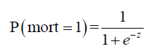
where z = b + w1 • age + w2 • lac + w3 • wbc + w4 • sexMale + w5 • typeMed + w6 • typeSurg
Instead of using the conventional mean squared error, we use a cost function called Cross-Entropy, also known as Log Loss. Cross entropy consists of two parts: one for mort =1 and the other for mort = 0. A cost function basically tells us how good our model is at making predictions for a given value of W and b.
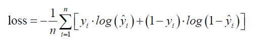
where  is the observed outcome which takes values of 0 or 1;
  is the predicted probability of event taking values from 0 to 1
 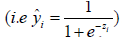 . With cross entropy, as the predicted probability comes closer to 0
  for the “yes” example
  , the loss increases closer to infinity. The purpose of model training is to find appropriate weights (W) and bias (b) to minimize the loss function.

The tf$matmul() function multiply two matrix X and W, note that the second dimension of X must be equal to the first dimension of W according to the matrix multiplication rule. Then the tf$add() function add the bias term b, resulting in a tensor in logit scale. The tf$nn$sigmoid() function is employed to transform the logit scale to probability. The next step is to define the loss function. We will use sigmoid cross entropy with logits as a loss function.

With the loss function being defined, we can use gradient descent approach to find appropriate weights and bias to minimize the loss function. The gradient measures how much the output of a function changes if you change the input a little bit. It can be thought of as the slope of a function. A higher gradient means a steeper slope and the faster a model can learn. In mathematical terms, a gradient is a partial derivative of the loss function with respect to its weights (6). The gradient of the loss function can be written as  w.r.t. the weights. The learning rate η determines the size of the step we take to reach the minimum. The update process can be written as:
  . The process can be written in R code as follows:

The second line defines an operation to initialize global variables in the graph. Now that we have trained the model, let’s evaluate it:

Save all values of model performance
There is a special operation called summary in TensorFlow™ to facilitate visualization of the model parameters like weights and biases of a logistic regression model, metrics like loss or accuracy values, and images like input images to a neural network. The summary operation takes in a regular tensor and outputs the summarized data to the computer disk.

The tf$summary$scalar() function is to write the values of a scalar tensor that changes over time or iterations to the computer disc. In the example, the loss and accuracy of the model performance are scalar tensors that change over training iterations. Similarly, the tf$summary$histogram() function is used to plot the histogram of the values of a non-scalar tensor. This gives us a view of how does the histogram (and the distribution) of the tensor values change over training iterations. In the example, it's used to monitor the changes of weights and biases distributions. The last line of code merges all statistics so that all summaries can be run at once within the running session.
Execute a graph within a session
Now that we have structured the graph, let’s execute a graph within a session. Note that all results can only be returned after running a session. Technically, a session places the graph operations on hardware such as CPUs or GPUs and provides methods to execute them.

The output shows that the accuracy is only 0.758, which is far less than that obtained by the conventional glm() function. We need to tune the hyperparameters to obtain a better predictive performance.
Hyperparameters
There are many hyperparameters in model training. Here we will explain some important ones for the logistic regression model.
- Epoch is one forward pass and one backward pass of all the training examples.
- Batch size is the number of training examples in one forward/backward pass. The larger the batch size, the more memory space you’ll need.
- Iteration is one forward pass and one backward pass of one batch of subjects in the training set.
Now let’s define some values for these important hyperparameters.

The display_freq_iter and display_freq_epoch are parameters for printing results during the training iterations. They will not influence the results. The above specification results in a total of 46 iterations.

Create an interactive session
An alternative method to run a session is by calling the tf$InteractiveSession() function. The only difference with a regular Session is that an InteractiveSession installs itself as the default session on construction. In other words, the InteractiveSession supports less typing, as allows to run variables without needing to constantly refer to the session object. In the example, we launch an InteractiveSession:

TensorBoard
TensorBoard is a visualization tool that comes with any standard TensorFlow™ installation. In Google’s words: “The computations you’ll use TensorFlow for (like training a massive deep neural network) can be complex and confusing. To make it easier to understand, debug, and optimize TensorFlow programs, we’ve included a suite of visualization tools called TensorBoard.” The two most important purposes of TensorBoard is: (I) to visualize the graph and (II) writing summaries to visualize the learning process. For example, the changes of accuracy across training epochs can be visualized with TensorBoard.
To visualize the graph with TensorBoard, we need to write log files of the program. To write event files, we first need to create a train_writer for those logs, using this code:

The directory stores log files and the graph of the program is added by using the add_graph() function. We will not call the tensorboard() function at present because we want to store more summary statistics to the train_writer object.
Run the model within a session
We need to initialize all variables at the beginning of running a session.

All used global variables need to be initialized (i.e., you do not need to initialize variables that are not run, or none of the runs depends on them.). The number of iterations is explained as above.

The above code loops through epochs. Recall that we have defined the total number of epochs to be 10,000. There are a number of iterations within each epoch. The actual data are passed to the sess$run() function by using the dict() function. The tensor objects (merged and optimizer) in the list argument are the part of the graph that run in the session. It is not necessarily to run the whole graph. The above loop print validation loss and accuracy at a frequency of 1,000 epochs, and at an iteration of 10 within each epoch. The output for the last training epoch is as follows:

Model validation in the testing set
Note that the model is evaluated in the validation cohort in the above session run, we can validate the model performance in the testing set as follows:

The first two lines transform the testing set to those suitable for passing to the TensorFlow™ placeholder. In the following sessions, we only run the loss and accuracy tensors because we already have trained the model with updated weights and bias. The result showed that the accuracy of the model was 0.93 in the testing set.
Weights and bias
The weights and bias after training can be obtained by running the b and W tensors in the session. Also remember to close the session after running.

The output shows that the weights and bias are close to the one obtained by the glm() method. However, you need to tune the hyperparameters such as learning rate and the number of epochs to achieve the minimal loss.
Launch the TensorBoard
The tensorboard() function provides a tool to inspect and understand your TensorFlow runs and graphs. The argument log_dir is to specify the directory to scan for training logs.

The TensorFlow™ graph is shown in Figure 2. The graph displays the tensors and operations defined in the previous code. From the bottom, there is a matrix multiplication between X and weights (W), and then the bias (b) was added. The tensor shape is shown in the data flow edge. In the scalar tab of the TensorBoard, there are two plots showing the accuracy and loss across training epochs. It appears that the training accuracy and loss stabilize after 5,000 epochs (Figures 3 and 4).


Concluding remarks
The article shows how to perform logistic regression model training in TensorFlow™ within R. It is useful for beginners who are going to work with TensorFlow™. However, the power of TensorFlow™ is not fully demonstrated with the current example (i.e., the accuracy of the model trained with TensorFlow™ is no better than the one trained with the conventional method). It is probably due to the fact that the data is simulated with generalized linear model and there is no complex interaction and non-linear terms. Thus, the maximum likelihood method is capable to obtain the weights and bias to maximize the likelihood function. Since the function is linear with monotone property, there is no local minima. TensorFlow™ has the power to model complex relationship among features and labels and it has been widely used for some deep learning methods. Understanding how the TensorFlow™ works will help to explore more on data science.
Acknowledgments
None.
Footnote
Conflicts of Interest: The authors have no conflicts of interest to declare.
Ethical Statement: The authors are accountable for all aspects of the work in ensuring that questions related to the accuracy or integrity of any part of the work are appropriately investigated and resolved.
References
- Tolles J, Meurer WJ. Logistic Regression: Relating Patient Characteristics to Outcomes. JAMA 2016;316:533-4. [Crossref] [PubMed]
- Shi L, Wang XC. Artificial neural networks: Current applications in modern medicine. IEEE, 2010:383-7.
- Chen JH, Asch SM. Machine Learning and Prediction in Medicine - Beyond the Peak of Inflated Expectations. N Engl J Med 2017;376:2507-9. [Crossref] [PubMed]
- Castelvecchi D. Can we open the black box of AI? Nature 2016;538:20-3. [Crossref] [PubMed]
- Stefaniak B, Cholewiński W, Tarkowska A. Algorithms of Artificial Neural Networks - Practical application in medical science. Polski Merkuriusz Lekarski. 2005;19:819-22. [PubMed]
- Ruder S. An overview of gradient descent optimization algorithms. Vol. cs.LG, arXiv.org. 2016.

