
An artificial intelligent platform for live cell identification and the detection of cross-contamination
Introduction
Cell line cross-contamination and misidentification have become serious problems since the first cross-contaminated HeLa cell line was reported in the 1950s (1,2). To date, one-fifth to one-third of cell lines have been cross-contaminated, which is commonly due to mislabeling, the repeated use of pipets, and the sharing of culture media (3-5). Cell line cross-contamination is often not readily detectable, resulting in inaccurate experimental results and unusable therapeutic products. The International Cell Line Authentication Committee, the National Institutes of Health, and many authoritative journals strongly urge researchers to authenticate cultured cells before carrying out experiments (6-8).
Various molecular approaches have been developed to distinguish different cell lines with respective strengths and limitations (3,9). Currently, the most frequently recommended method is short tandem repeat (STR) profiling, which detects variations in the number of STR sequences within microsatellite DNA (10). Each of the repeat regions is amplified and compared with the standardized cell line profiles. In general, 80% similarity is the threshold for declaring a match (10,11). However, the application of STR is limited by its high cost and availability only in specialized institutions. STR profiling is only suitable for distinguishing cell lines of a single species and is affected by genetic drift (12). Karyotyping (13) and polymerase chain reaction (14) can separate species as supplemental techniques. Single-nucleotide polymorphism and whole-genome sequencing are less affected by genetic drift but are very expensive (15). Moreover, complex expertise is required for each technology. In contrast, observation of morphology is a simple and direct technique to characterize cell lines. Cultured cells can be morphologically divided into three basic categories: fibroblast-like (elongated), epithelial-like (polygonal), and lymphoblast-like (spherical). However, whether cell morphology can be used to separate individual cell lines for cell identification is unclear.
Deep convolutional neural networks (CNNs) are widely used in modern artificial intelligence (AI), and have been successfully applied in medical image classification, including the identification of skin cancer (16) and retinopathy (17). Additionally, CNNs can analyze live cell images for mitosis detection (18) and hematopoietic lineage tracing (19). Moreover, their superiority in semantic segmentation that outputs pixel-wise predictions increase the precision of image recognition (20). CNNs provide new insights into individual cell lines identification and cross-contamination detection by morphological identification.
In this study, we sought to classify cell lines with similar morphologies and to identify cross-contaminated cells by a novel AI platform with three deep learning networks, AlexNet, bilinear CNN (BCNN), and DilatedNet. Specifically, we obtained microscopy images of seven commonly used cell lines to train these deep learning models, and applied eight categories of co-cultured cell lines (mixing two of the seven) for model testing.
Methods
Cell culture and image acquisition
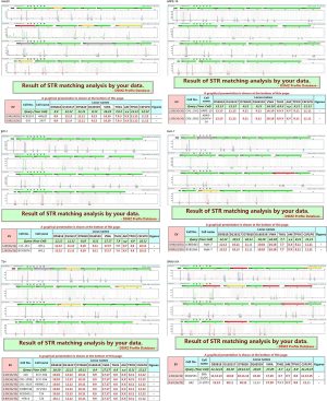
Strict cell culture practices were utilized to prevent accidental co-culture among these seven cell lines, as follows: (I) handling one cell line at a time; (II) keeping each medium in a separate container; (III) carefully labeling each culture flask with the cell line name, passage number, and operation date; and (IV) discarding pipettes in a timely manner after each operation. The conditional medium that was used is provided in Table S1. Cells were seeded from low to intermediate density and were cultured in a humidified atmosphere of 5% CO2 at 37 °C. Continuous passage-culture was conducted for 10 passages. Images were acquired using an inverted phase-contrast microscope (Carl Zeiss Axio Vert A1). Each image was obtained at 50× optical magnification with a size of 1,040×1,388 pixels. The STR analysis was conducted by Sun Yat-sen University Forensic Medical Center (Figure S1). Eight types of cell mixtures were co-cultured as indicated in Table S1. The cells were seeded at a density in a mixture ratio of 1:10 to 1:1,000. Images were taken every day.
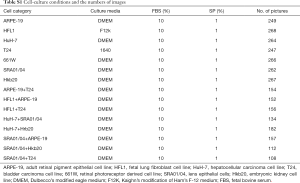
Full table
Preprocessing
The preprocessing of cell microscopy images mainly focused on improving the image quality and reducing the effect of noise. First, Gauss filtering was performed. Then, to avoid the impact of an imbalanced background light on the prediction results and to improve the robustness of the method, we employed gray normalization for brightness balance and contrast enhancement of the cell microscopy images using the following formula:
|
| [1] |
Where Iin is the gray value of the pixel in the input image, Iout is the gray value of the pixel in the output image, Meanin and STDin are the mean and standard deviation, respectively, of the input image, and Meanout and STDout are the mean and standard deviation of the image after normalization. In this work, we set Meanout and STDout to 180 and 20, respectively.
Data augmentation
Data augmentation is essential for teaching the network the desired invariance and robustness properties. For microscopy images, we primarily need cell size invariance and robustness against gray value variations. We employed two distinct forms of data augmentation. The first form of data augmentation is cell image scaling, which can ensure that the model obtains a certain degree of cell size invariance. The second form of data augmentation is gamma correction, as shown in the following formula; the model can learn the illumination invariance by adjusting the brightness of the original training set image to different ranges.
|
| [2] |
Where r is the input image gray level, s is the output image gray level, and c and γ are constants.
Cell density effect
Cell morphology will differ when the density of cells varies. This variation could affect the performance of the model. Thus, an effective method for measuring cell density is necessary. For the gray-normalized cell microscopy images, we employed the adaptive threshold processing method and morphological operations to generate a cell region mask image. Each pixel had a value of 0 or 1, with 0 indicating that the pixel was the background and 1 indicating the cell region. The cell density was then calculated by the proportion of the cell regions as the following formula.
|
| [3] |
To explore the effect of cell density on the performance of the model, we partitioned the dataset using a fixed cell density threshold. We then, chose the same numbers of high- and low-density cell images to make up the training dataset. We used high- and low-density cell microscopy images to train the models, with the other parameters remaining exactly the same. We then tested the performance of the high- and low-density models on test sets with all densities. The effect of cell density on the accuracy of the model was evaluated.
AlexNet
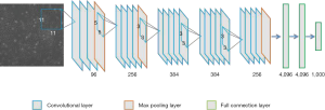
We used AlexNet as the CNN model for initial cell classification. AlexNet is a pioneering deep CNN that won the ILSVRC-2012 with a top-5 test accuracy of 84.6%. The architecture is relatively simple and consists of 5 convolutional layers, max-pooling layers, rectified linear units (ReLUs) as non-linearities, three fully connected layers, and a dropout. Figure S2 shows the CNN architecture.
Bilinear CNN model
The BCNN (21) for image classification consisted of a quadruple B = (fA; fB; P; C). Here, fA and fB are feature functions based on CNNs, P is a pooling function, and C is a classification function. A feature function is a mapping, which takes an image and a location L and outputs a feature of size K×D. The location can include position and scale. The feature outputs are combined at each location using the matrix outer product. That is, the bilinear combination of fA and fB at location l is given by
|
| [4] |
In this work, we used VGG16 truncated at relu5_3 (22) as the feature function. The input image block size was 192×192 pixels, and proceeding through VGG16 produced 12×12×512-pixel features. Then, the feature map was reshaped to 144×512 pixels. The feature vector was multiplied by its transposition using the outer product at each location of the cell image to obtain the bilinear vector. The bilinear vectors were fed to a two-layer fully connected layer of dimension 1,024 and 7 (cell categories) respectively.
Dilated network
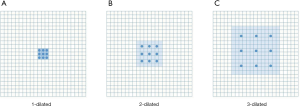
Dilated (23) convolutions are a generalization of Kronecker-factored convolutional filters, which support exponentially expanding receptive fields without losing resolution.
Let F: Z2→R be a discrete function. Let Ωr = [−r, r]2 ∩ Z2 and let k: Ωr→R be a discrete filter of size (2r+1)2. The discrete convolution operator * can be defined as
|
| [5] |
We now generalize this operator. Let l be a dilation factor, and let *l be defined as
|
| [6] |
We will refer to *l as a dilated convolution or a l− dilated convolution. The familiar discrete convolution * is simply the 1− dilated convolution.
Results
Image acquistion, preprocessing and augmentation
Seven commonly used cell lines, including epithelial cells (SRA01/04, ARPE19, and Hkb20), fibroblasts (HFL1), nerve cells (661W), and tumor cells (HuH-7 and T24), were cultured and verified by STR analysis (Figure S1). Pure-cell images were taken from independently cultured cell lines (a total of 1,823 images) for model training, which was conducted by six-fold cross-validation. Pure-cell images as well as images from eight categories of co-cultured cell lines (mixing two of the seven and a total of 848 images) were used for model testing (Table S1). All images were captured with 50× optical magnification at a size of 1,040×1,388 pixels.
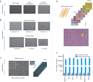
To improve image quality and reduce noise, we performed gray normalization and contrast enhancement (see Methods). Given the potential variations in size and background brightness, we performed gamma correction and imaging scaling on the captured pure-cell images before model training (Figures 1A,B). After preprocessing and data augmentation, we used a sliding window (192×192 pixels, with a 64-pixel striding step) to scan the pure-cell images and segment them into patches for model training (Figure 1C). The patches were classified and assigned a corresponding color. To determine the final classification of the raw image data, we returned the pseudo-colored patches to their original locations and generated a heat map. The most prevalent patch was regarded as the final classification of the entire image (Figure 1D). This process increased the number of training sets to 333,862–362,247 pieces per cell and to a total of 2,464,090 pieces for all seven cell lines (Figure 1E). The risk of overfitting was also reduced by this data expansion approach (24).
Classification of pure-cell images using AlexNet
The application of AlexNet (25) using the CNN method has increased the accuracy of traditional machine learning models from 70% to 80%. Compared to the other networks with hundreds to thousands layers, AlexNet contains only 8 layers, resulting in the network’s ease of operation and minimal calculation requirements (Figure S2).
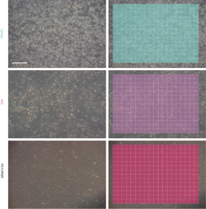
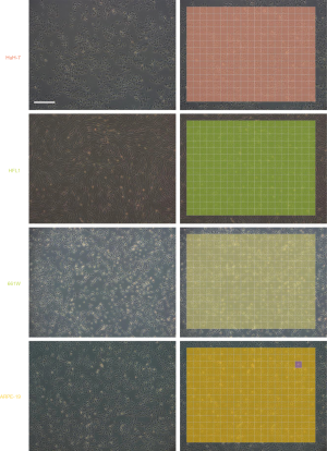
First, we trained the AlexNet classifier to identify the seven pure cell lines. The agreement between the ground truth and the test results was 98.9% in the test set (the mean of all classes), and the confusion matrix is shown in Figure S3. After returning the pseudo-colored patches to their original locations, most pure-cell images for testing resulted in a homochromatic heat map with their corresponding colors. The classification result of an entire image is shown in Figure 2 and Figure S4.
The shape and size of the cells can be affected by cell density. To test whether cell density affects the accuracy of the model, we implemented pure cell line images with low- and high-cell density for AlexNet-based model training. The low-density cell model performed well with the low-cell-density (0–50% confluence) part of the validation set (average accuracy of 94.74%), and the high-density model performed well in the high-cell-density (50–100% confluence) part of the validation set (average accuracy of 97.23%). The accuracy of the high-density model on cells with lower than 20% confluence (accuracy of 58.77%) was higher than that of the low-density model on cells with higher than 80% confluence (accuracy of 25.3%) (Figure 3A). These results suggest that high- and low-density cell images had different features, that images of both cell densities are necessary for model training, and that AlexNet performed better with high-cell-density images. This was likely because high-density images contained more cells in each patch. Moreover, high-density cells were not simply closer together but rather presented a texture that may be a key feature the AI extracted (26,27).
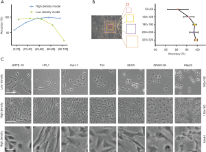
The size of the sliding window can also affect the accuracy of the model, as a larger window will contain a larger number of cells with a more complex texture of patches. Therefore, we tested the model classification accuracy with window sizes of 64×64, 128×128, 192×192, 256×256, and 320×320 pixels. The accuracy of the model was greater than 97% with a window size of 192×192 pixels, and 99% with a window size of 320×320 pixels, indicating that the accuracy of classification improved as the window size increased (Figure 3B,C).
Detection of cross-contamination and identification of cell types using multiple models
Eight data sets of images with two different co-cultured cell types were obtained. The first step for the AI model was to determine whether the cells were pure or mixed. After scanning, the entire image was divided into patches (a heat map). We took the maximum proportion possessed by any patch type as the probability of a pure cell population (Figure 4A). To get an appropriate threshold, we tested on both pure-cell and contaminated-cell datasets and drew a receiver operating characteristic (ROC) map, which showed that the classifier had excellent performance, with an area under the ROC curve (AUC) of 0.9872. According to the ROC curve, we set the classification threshold of 97.37%, with the true positive rate of 90.86% and the false positive rate of 2.54% (Figure 4A). If the maximum proportion of the resulting color was greater than the threshold, we directly used the maximum patch result as the cell identity and compared this result with the original cell tag to determine whether the label was correct. If the sample was contaminated, the potential type of candidate cell was suggested according to the classification result. We calculated the identification accuracy as A or B in the mixed-cell (A + B) test set (Figure S7) and found an average accuracy of 67.66%, indicating that AlexNet could not accurately differentiate mixed cells.
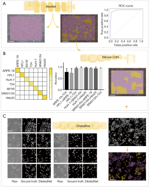


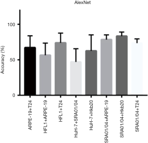
Since the identification of mixed cells was based on the classification of pure cells, we further improved the accuracy of the model in recognizing the seven pure-cell types. Actually, cell type classification is a type of fine-grained image classification, which aims at recognizing sub-categories within a same basic category, such as granite and marble. The texture features of images are the key factors in fine-grained identification (28), which is also consistent with our analysis of image features by density and window-size testing above. Recently, Lin et al. proposed an end-to-end architecture for fine-grained visual recognition called BCNN, which achieved the best classification accuracy for the CUB200-2011 dataset among weak supervised fine-grained classification models (21). The extracted features can be presented as an outer product of two features, f(A) and f(B), extracted from a standard CNN.
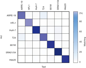
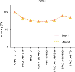
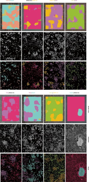
A pre-trained visual geometry group network (VGG-16) was taken as a standard CNN. Before the fully connected layer, a specially designed bilinear vector was obtained via multiplication using the outer product from the concatenation of the last feature maps and its transposition. The architecture of BCNN is based on Tensorflow (Figure S5). Training was performed by stochastic gradient descent (SGD) with a mini-batch size of 16 and momentum of 0.9. In total, 100,000 iterations were performed with a learning rate of 10-4. We performed tests with the pure-cell dataset and the mixed-cell dataset. The average accuracy of the BCNN model (pre-trained VGG-16 with a bilinear vector) for the pure-cell test dataset was 99.5%, and the relative confusion matrix for the pure-cell test set is shown in Figure 4B. The BCNN model achieved a mean accuracy of 86.26% for the mixed-cell test dataset, which was significantly higher than that of AlexNet (Figure 4B, Figure S8). Moreover, the pre-trained VGG-16 achieved 74.51% mean accuracy on the mixed-cell dataset. To improve the visualization resolution, we modified the step size of the sliding window from 64 to 1 to locate the edges, which represent the output with 64×64 or 1×1 in the center of each sliding window; however, the average accuracy did not significantly change (Figure 4B, Figure S9).
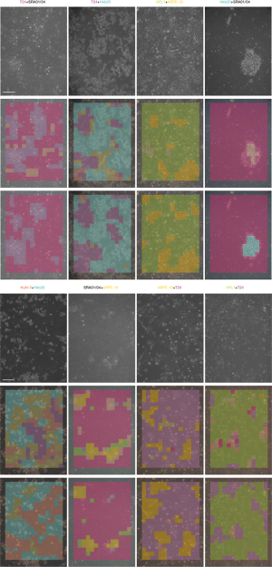
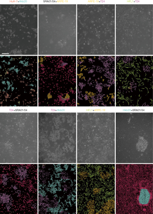
Smantic segmentation algorithm was applied to distinguish cells from background and divide them into single cells with clear boundaries. Conventional semantic segmentation networks such as fully convolutional networks (FCN) (29), SegNet (30) and U-net (31) integrate multi-scale contextual information via successive pooling and upsampling layers that reduce resolution. However, in our case, the features of edges, which are small but important for cell segmentation, might be lost because of pooling and upsampling. Dilated convolution has an unchanged kernel with an exponentially increased receptive field. We constructed a 10-layer neural network called DilatedNet based on dilation convolution that only contained convolution layers without pooling or upsampling (Figures S6,S10). We then implemented DilatedNet using Tensorflow and Keras and labeled 1,200 single cell images with 512×512 pixels. The cell images and labels were divided into a training set, a validation set, and a test set in a 4:1:1 ratio. Model training was performed by Adam (32) with a mini batch size of 5. In total, 100,000 iterations were performed, with a learning rate of 1e-4. DilatedNet achieved an accuracy of 98.2% on the test set. The segmentation result is shown in Figure 4C. Then, we merged the cell types (the classification result using BCNN) and cell locations (the segmentation result using DilatedNet) as the final representation of the mixed-cell data set (Figure 5, Figure S5). Therefore, cross-contamination can be shown at the individual-cell level.
Discussion
This study is the first to detect cross-contaminated or misidentified cell lines using a deep learning technique combining AlexNet, BCNN and DilatedNet. AlexNet achieved an AUC of 0.9872 for detecting contamination. BCNN achieved an accuracy of the model for classification of 99.5% for the seven pure cell lines and an accuracy of 86.3% for the eight categories of co-cultured cell lines (mixing two of the seven). DilatedNet was applied to the semantic segment for each single cell with precise edges and achieved an accuracy of 98.2% on the test set. We also characterized how CNN differentiated cell images with similar morphologies by the density test and the window-size test. Our results suggest that despite the single-cell size and shape characteristics, textures formed by growth are also important morphological features. Our findings also help improve the classification through the fine-grained identification network.
Cell lines undergo genetic drift with continued passaging in culture due to changes in allele frequencies that occur in random sampling of the parent. Genetic drift may lead to deletion or mutation of certain alleles and may be accentuated by overpassaging or overdiluting, especially for malignant cell lines (3). This cell line instability can lead to changes in STR markers such as satellites, reducing the specificity of STR analysis. As a result, STR sets a threshold of 80% to allow a certain degree of genetic drift. Several studies have found that cell lines at high passage numbers experience morphological changes (33). The SNP test, which is less affected by genetic drift (34), can be applied to determine whether a cell line will spontaneously change its identity during long-term culture. Subsequently, we can collect cell images before and after an identity change to train a more accurate AI platform.
Studying one disease in vitro often involves only a few cell lines. This study successfully completed the test of seven types of cell lines that are suitable for specialist laboratories. In the future, modules that are classified according to anatomical systems can be built and tested in specific research areas. In addition, this AI system has basically covered all current ophthalmic cell lines.
Online detection and cloud updates may provide better user experience and system optimization. After uploading the images to be detected to the website, the test result can be directly obtained, and the uploaded images will be used for a new round of training. Moreover, the exclusive AI identification system can be customized, especially in the case of newly established or purchased cell lines. It was important to note that new cell types need to be certified by STR before training the customized model. Because cell images have similar underlying features, custom models will be trained more efficiently by transfer-learning methods based on existing models. For cell banks that manage thousands of cells, completing a large number of classifications at the same time may require more powerful hardware to support the computation of large data, which requires more cooperation to achieve. In the other side, collecting thousands of types of cell images is an irreplaceable advantage of the cell banks.
We demonstrated that BCNN is particularly useful for fine-grained classification on when testing mixed-cell images, which can model local pairwise feature interactions in a transnationally invariant manner. In contrast, the traditional classification neural networks, such as AlexNet, are designed for classification of large objects (e.g., birds, flowers, and dogs) and may not be suitable for small objects with distinct textural features. The main idea of BCNNs is the bilinear vector, the possible explanation of its “black box” is two mutually coordinated components: f(A) targeted the location of objects, whereas f(B) extracts their features. In addition, BCNN was based on a pre-trained VGG-16, one of the most widely used CNNs. Compared with AlexNet, VGG has a deeper architecture. Based on transfer learning, a pre-trained VGG-16 can be used rather than training a completely blank network.
Proximity to the image input layer corresponds to more extracted features shared in common, whereas the deeper layers extract more advanced, abstract, and task-specific features. Therefore, we can keep the parameters of the shallow layers unchanged and retrain the deeper layers to solve our own classification tasks. With this fine-tuning approach, we can save more computational power and achieve decent prediction accuracy while using a larger network. In this study, the pre-trained VGG-16 increased the accuracy for AlexNet significantly by 6.85%. Based on the pre-trained VGG, the bilinear vector contributed an additional 12% accuracy.
The classification results of mixed-cell images could not be shown as individual cells using the BCNN, so a dilated convolutional network was used to separate the cells. In addition, we tried some semantic segmentation networks used for natural scenes (U-net, Seg-net, and FCN) to achieve segmentation and classification in one step. However, these semantic segmentation networks did not perform well in our dataset, exhibiting a relatively high loss rate. Their purpose is to achieve segmentation and classification in one step, but they did not perform well in this dataset. The probable reason was that these networks often show a loss of edge in objects. When using individual cells for training, loss of edges is not acceptable for such tiny cells.
In summary, we successfully demonstrated that CNNs can be trained by images of pure cell lines to determine misidentification and cross-contamination of live cultured cell lines. This AI system requires no reagents and can be performed in house and in real time. The system is readily available, allowing faster popularization, and can provide wider coverage with powerful efficacy. However, further work is necessary to determine the feasibility of applying this model to authenticate thousands of cell lines.
Acknowledgments
Funding: This study was funded by the National Key R&D Program of China (2018YFC0116500), National Natural Science Fund for Distinguished Young Scholars (81822010).
Footnote
Provenance and Peer Review: This article was commissioned by the Guest Editors (Haotian Lin and Limin Yu) for the series “Medical Artificial Intelligent Research” published in Annals of Translational Medicine. The article was sent for external peer review organized by the Guest Editors and the editorial office.
Conflicts of Interest: All authors have completed the ICMJE uniform disclosure form (available at http://dx.doi.org/10.21037/atm.2019.07.105). The series “Medical Artificial Intelligent Research” was commissioned by the editorial office without any funding or sponsorship. HL served as the unpaid Guest Editor of the series. The other authors have no other conflicts of interest to declare.
Ethical Statement: The authors are accountable for all aspects of the work in ensuring that questions related to the accuracy or integrity of any part of the work are appropriately investigated and resolved.
Open Access Statement: This is an Open Access article distributed in accordance with the Creative Commons Attribution-NonCommercial-NoDerivs 4.0 International License (CC BY-NC-ND 4.0), which permits the non-commercial replication and distribution of the article with the strict proviso that no changes or edits are made and the original work is properly cited (including links to both the formal publication through the relevant DOI and the license). See: https://creativecommons.org/licenses/by-nc-nd/4.0/.
References
- Gartler SM. Apparent HeLa Cell Contamination of Human Heteroploid Cell Lines. Nature 1968;217:750-1. [Crossref] [PubMed]
- Lande R. Natural Selection and Random Genetic Drift in Phenotypic Evolution. Evolution 1976;30:314-34. [Crossref] [PubMed]
- Capes-Davis A, Theodosopoulos G, Atkin I, et al. Check your cultures! A list of cross-contaminated or misidentified cell lines. Int J Cancer 2010;127:1-8. [Crossref] [PubMed]
- Neimark J. Line of attack. Science 2015;347:938-40. [Crossref] [PubMed]
- Horbach SPJM, Halffman W. The Ghosts of HeLa: How cell line misidentification contaminates the scientific literature. PLoS One 2017;12:e0186281. [Crossref] [PubMed]
- Lorsch JR, Collins FS, Lippincott-Schwartz J. Fixing problems with cell lines. Science 2014;346:1452-3. [Crossref] [PubMed]
- Masters JR. Cell-line authentication: End the scandal of false cell lines. Nature 2012;492:186. [Crossref] [PubMed]
- Nardone RM. Eradication of cross-contaminated cell lines: A call for action. Cell Biol Toxicol 2007;23:367-72. [Crossref] [PubMed]
- Almeida JL, Cole KD, Plant AL. Standards for Cell Line Authentication and Beyond. Plos Biol 2016;14:e1002476. [Crossref] [PubMed]
- Masters JR, Thomson JA, Daly-Burns B, et al. From the Cover: Short tandem repeat profiling provides an international reference standard for human cell lines. Proc Natl Acad Sci 2001;98:8012-7. [Crossref] [PubMed]
- Lorenzi PL, Reinhold WC, Varma S, et al. DNA fingerprinting of the NCI-60 cell line panel. Mol Cancer Ther 2009;8:713-24. [Crossref] [PubMed]
- Poetsch M, Petersmann A, Woenckhaus C, et al. Evaluation of allelic alterations in short tandem repeats in different kinds of solid tumors—possible pitfalls in forensic casework. Forensic Sci Int 2004;145:1-6. [Crossref] [PubMed]
- MacLeod RA, Kaufmann M, Drexler HG. Cytogenetic harvesting of commonly used tumor cell lines. Nat Protoc 2007;2:372-82. [Crossref] [PubMed]
- Liu M, Liu H, Tang X, et al. Rapid identification and authentication of closely related animal cell culture by polymerase chain reaction. In Vitro Cell Dev Biol Anim 2008;44:224-7. [Crossref] [PubMed]
- Didion JP, Buus RJ, Naghashfar Z, et al. SNP array profiling of mouse cell lines identifies their strains of origin and reveals cross-contamination and widespread aneuploidy. BMC Genomics 2014;15:847. [Crossref] [PubMed]
- Esteva A, Kuprel B, Novoa RA, et al. Dermatologist-level classification of skin cancer with deep neural networks. Nature 2017;542:115-8. [Crossref] [PubMed]
- Gulshan V, Peng L, Coram M, et al. Development and Validation of a Deep Learning Algorithm for Detection of Diabetic Retinopathy in Retinal Fundus Photographs. JAMA 2016;316:2402-10. [Crossref] [PubMed]
- Held M, Schmitz MHA, Fischer B, et al. CellCognition: time-resolved phenotype annotation in high-throughput live cell imaging. Nat Methods 2010;7:747-54. [Crossref] [PubMed]
- Buggenthin F, Buettner F, Hoppe PS, et al. Prospective identification of hematopoietic lineage choice by deep learning. Nat Methods 2017;14:403-6. [Crossref] [PubMed]
- Hao X, Zhang G, Ma S. Deep Learning. IEEE Trans Pattern Anal Mach Intell 2016;10:417-39. [PubMed]
- Lin TY, Roychowdhury A, Maji S. Bilinear CNNs for Fine-grained Visual Recognition. In ICCV, 2015.
- Simonyan K, Zisserman A. Very Deep Convolutional Networks for Large-Scale Image Recognition. In ICLR, 2015.
- Noh H, Hong S, Han B. Learning deconvolution network for semantic segmentation. Proc IEEE Int Conf Comput Vis 2015.1520-8.
- Guo J, Gould S. Deep CNN ensemble with data augmentation for object detection. arXiv preprint arXiv:1506.07224, 2015.
- Krizhevsky A, Sutskever I, Hinton G E. Imagenet classification with deep convolutional neural networks. In NIPS, 2012.
- Haralick RM, Shanmugam K, Dinstein IH. Textural Features for Image Classification. IEEE Trans Syst Man and Cybernet 1973;3:610-21. [Crossref]
- Xie Y, Wang J. Study on the identification of the wood surface defects based on texture features. Optik - Int J Light Electron Opt 2015;126:2231-5. [Crossref]
- Lowe DG. Object recognition from local scale-invariant features. ICCV 1999;99:1150-7.
- Long J, Shelhamer E, Darrell T. Fully convolutional networks for semantic segmentation. In CVPR, 2015: 3431-40.
- Badrinarayanan V, Kendall A, Cipolla R. Segnet: A deep convolutional encoder-decoder architecture for image segmentation. IEEE Trans Pattern Anal Mach Intell 2017;39:2481-95. [Crossref] [PubMed]
- Ronneberger O, Fischer P, Brox T. editors. U-Net: Convolutional Networks for Biomedical Image Segmentation. International Conference on Medical Image Computing & Computer-assisted Intervention; 2015.
- Kingma D, Ba J. Adam: A Method for Stochastic Optimization. Comput Sci 2014;43:87-4.
- Hughes P, Marshall D, Reid Y, et al. The costs of using unauthenticated, over-passaged cell lines: how much more data do we need? Biotechniques 2007;43:575-577-8, 581-2 passim. [Crossref] [PubMed]
- Castro F, Dirks WG, Fähnrich S, et al. High-throughput SNP-based authentication of human cell lines. Int J Cancer 2013;132:308-14. [Crossref] [PubMed]


