

Predictive analytics with gradient boosting in clinical medicine
Introduction
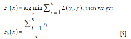
Predictive analytics play an important role in clinical research. If a clinical condition or outcome can be accurately predicted, interventions can be delivered to the patient population who will benefit the most. Thus, numerous data mining algorithms have been developed for clinical prediction in nearly all subspecialties. However, the most widely used method for making clinical predictions is the generalized linear model (GLM). The shortcomings of this method include, but are not limited to, linearity and additivity assumptions. In a hypothesis-driven framework, GLM methods are amiable to researchers because the trained model is relatively easy to understand and interpret.
However, with the development of electronic healthcare records, a large amount of healthcare data is readily available to clinical investigators. These often have latent complex relationships among particular variables which may not even be considered hypothetically by the investigators developing their predictive models. Machine learning methods can be used in this setting as we can rely on the predictive algorithm to discover the nonlinearity and interaction structure in the data instead of hoping that the investigators will be wise enough to include such structure explicitly in their models.
Among the many machine learning techniques, gradient boosting is a particularly attractive approach. It was first introduced in 1999 by Stanford University Professor Jerome H. Friedman (1) and has been further developed and refined in several open source packages such as Scikit-Learn, and R. Major software developers such as SAS and IBM have developed their own implementations and Friedman’s original gradient boosting machine (with refinements) has been part of the Salford Systems SPM product since 2001. As of early 2019, Google scholar reports about 10,000 citations in the scientific literature to Friedman’s two papers introducing gradient boosting and applications can be found in almost all fields of scientific investigation.
In the clinical literature, gradient boosting has been successfully used to predict, among other things, cardiovascular events (2), development of sepsis (3), delirium (4) and hospital readmissions following lumbar laminectomy (5). However, the methodology is not well known among clinicians. Thus, this article aims to provide a practical guide on how to perform gradient boosting using R.
How gradient boosting works
Before we talk about the concept of gradient boosting, let’s look at a simple example that reveals the main idea of formal gradient boosting.
Traditionally, modelers would try to find a function that can accurately describe the data. However, the function can only be an approximation of the data distribution and there must be errors:

where yi is the outcome variable and Xi is a vector of predictors.
Suppose that the F1 (Xi) function is a weak learner and the relationship between X and y is not fully described. In this situation, the error or residual is not white noise but has some correlation with y. We may want to train a second model on the error term:

The updated model will look something like:

After performing this procedure iteratively we finally can fit a model at the Mth step:

Gradient boosting allows one to plug in any class of weak learners hm (Xi) to improve predictive accuracy. In other words, the hm (Xi) is a weak learner that can take any functional form such as a GLM, a neural network or a decision tree. Although there is no requirement for hM (Xi) to be a specific function, it is usually a tree-based learner in practice.
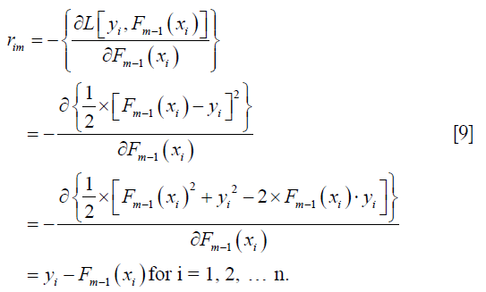
The residual or error can be expressed as the loss function L [Y, FM (X)] in machine learning terminology and our objective is to build a model that minimizes this loss. More formally, the loss function is defined as the difference between the predicted [FM (X)] and the observed value (Y). The loss function can be the squared error for an ordinary least squares regression model. For loss functions that cannot be resolved with simple algebra, gradient descent is commonly employed to estimate the optimal parameters.
Gradient descent is a first-order iterative optimization algorithm for finding the minimum of a function (6). Conventionally, the gradient is calculated with respect to the model parameter. In gradient boosting, the gradient of the loss function is calculated with respect to the predicted value. That is, one takes the derivative of the loss function with respect to the predicted value. The gradient can be considered as pseudo-residual. More formally, gradient boosting proceeds with the following steps (7):
- Initialize the model by solving the following equation:
- For m =1 to M
- Fit the weak learner hm (x) to the residuals by:
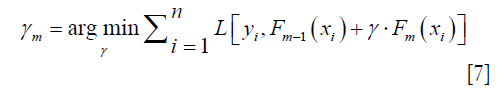
- Update the Fm (x) = Fm–1 (x) + γm · hm (x)
Compute the gradient with respect to predicted value,
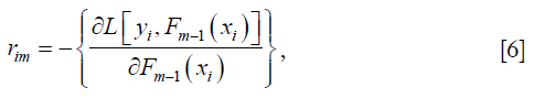
where i is the index for observations. Each observation will have one gradient value. The lowercase m is the number of boosting iterations with m ∈ [1, M].
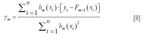
Computing the γm to solve the optimization problem:
By solving this equation we can get:
An illustrative example
To make sure one really understands gradient boosting approach, we’ve created an example which explains the intuition behind the method.
Suppose we want to predict systolic blood pressure based on one’s demographics including age, gender and obesity. Ten subjects are observed as follows:

The initial value for the F function is the mean. The squared error is used as the loss function, and the gradient of the loss function can be calculated as follows:
In the current iteration (m=1), the yi is the observed blood pressure (BP) for each individual. The Fm-1 (xi) is a vector of mean values of BP. The gradient (pseudo residual) can be computed with the following R code.

Note that the pseudo residual considers not only the direction but also the magnitude of the difference between the observed and predicted values. Next, we will fit a regression tree to the pseudo residual:

The maximum depth of the tree is set to two, making it a weak leaner. Because there are only ten observations, the minimum number of observations that must exist in a node in order for a split to be attempted is five. The prediction made by the regression tree is h1 which will be added to the F0 (X) to update it to calculate F1 (X):

Then the above process is repeated and the F1 (X) function can be updated to calculate F2 (X).

The above output shows how gradient boosting progresses from F0 to F2 and how the h0, pseudo residual, and F values change with fitting a regression tree to the gradient recursively. We can also visualize the regression tree with a couple of lines:

The terminal nodes of the left tree show the percentage and mean values, which is consistent with that shown in the above table (Figure 1). There are five subjects (3, 6, 7, 9 and 10) in the leftmost node. These are individuals with age <45 years. The prediction of BP with mean value of the overall population is too high. Thus, the updated F1 prediction is F0 minus 19.3, which is much closer to the true value.

For gradient tree boosting, a slightly modified algorithm is employed that uses a different γm for each leaf node, denoted as γjm for leaf node j.
Hopefully, one now has an intuition as to how gradient boosting works. Next, we will show you how to perform gradient tree boosting in practice with a simulated dataset.
Working example
A simulated dataset was created for the purpose of illustration. The following R code generate a dataset with three categorical (Ncat =3) and four continuous (Ncont =4) variables. The outcome variable Y is a binary variable with levels of 0 and 1. Note that the linear predictor is constructed with several interaction and quadratic terms.

Split the sample into training and testing subsamples
Throughout the rest of this paper, the caret package (v6.0-81) will be used for training gradient tree boosting (8).

The createDataPartition() function is used to split the dataset into training and testing subsamples. The first argument of the function is the outcome variable. Random sampling is done within the levels of Y in an attempt to balance the class distributions within the splits. The p argument specifies the percentage of data which goes into the training set. The function returns a matrix of row position integers corresponding to the training data.
Logistic regression model
A logistic regression model is first fit to the data to see whether the gradient boosting model is able to improve predictive performance when there are arbitrary interactions and non-linear terms among the covariates.

The output shows that the area under the receiver operating characteristic curve (AUROC) of the logistic regression model is 0.92 (95% CI: 0.87–0.97).
Gradient tree boosting

The trainControl() function controls many computational nuances of the train() function. In the example, ten-fold cross validation is carried out. Specifically, the whole data sample is randomly divided into ten blocks of roughly equal size. Each of the blocks is left out in turn and the other nine blocks are used to train the model. The held-out block is predicted on and these predictions are summarized into some type of performance measure such as accuracy for classification, and sum of squared error for regression. The above procedure is repeated ten times, resulting in 10×10=100 estimates of performance. These are then averaged to get the overall resampled estimate.

The expand.grid() function creates a data frame for all combinations of the supplied vectors or factors. Here we need to introduce a new term called a hyperparameter. The hyperparameters define how our model is actually structured. They are different from model parameters and cannot be trained from the data. Grid search is arguably the most basic hyperparameter tuning method. With this scheme, we simply build a model for each possible combination of all of the hyperparameter values provided, evaluate each model and select the architecture which produces the best results. The hyperparameters of decision tree modeling include the maximum depth of each tree (interaction.depth), number of trees (n.trees), learning rate (shrinkage) and the minimum number of observations in the terminal nodes of the trees (n.minobsinnode).

Finally, the model can be trained with the train() function. The training process can be viewed with the generic plot() function.

Figure 2 shows the training process with one grid searching strategy. The results indicate that the accuracy increases rapidly from iteration number 1 to 100, but then levels off after 100 iterations. A tree depth of more than three will not continue to improve predictive accuracy.


The result shows that AUROC of the gradient boosting model (0.98; 95% CI: 0.972–0.997) is significantly higher than the logistic regression model (with a P value of 0.008 using DeLong’s test).
Conclusions
Traditional statistical modeling has long been plagued by the assumption that the particular functional form of the relationship between the outcome and predictor variables has been accurately captured by the modeler. New data mining techniques, such as gradient boosting, allow algorithms to detect potentially latent variables such as interaction and higher order terms which are difficult to explicitly model.
This paper has illustrated a step-by-step approach to gradient boosting and shown that it can lead to higher predictive power in a simulated dataset than logistic regression. The authors hope that this paper will be useful to clinicians and other health care researchers who want to apply gradient boosting to their own data sets with the expectation of an increase in predictive power.
Acknowledgements
None.
Footnote
Conflicts of Interest: The authors have no conflicts of interest to declare.
References
- Friedman JH. Greedy function approximation: A gradient boosting machine. The Annals of Statistics 2001;29:1189-232. [Crossref]
- Zhao J, Feng Q, Wu P, et al. Learning from Longitudinal Data in Electronic Health Record and Genetic Data to Improve Cardiovascular Event Prediction. Sci Rep 2019;9:717. [Crossref] [PubMed]
- Delahanty RJ, Alvarez J, Flynn LM, et al. Development and Evaluation of a Machine Learning Model for the Early Identification of Patients at Risk for Sepsis. Ann Emerg Med 2019;73:334-44. [Crossref] [PubMed]
- Wong A, Young AT, Liang AS, et al. Development and Validation of an Electronic Health Record-Based Machine Learning Model to Estimate Delirium Risk in Newly Hospitalized Patients Without Known Cognitive Impairment. JAMA Netw Open 2018;1:e181018. [Crossref] [PubMed]
- Kalagara S, Eltorai AEM, Durand WM, et al. Machine learning modeling for predicting hospital readmission following lumbar laminectomy. J Neurosurg Spine 2018;30:344-52. [PubMed]
- Ruder S. An overview of gradient descent optimization algorithms. Vol. cs.LG, arXiv.org. 2016.
- Friedman JH, Meulman JJ. Multiple additive regression trees with application in epidemiology. Stat Med 2003;22:1365-81. [Crossref] [PubMed]
- Kuhn M. caret: Classification and Regression Training. Available online: https://CRAN.R-project.org/package=caret. 2017.

