
Estimate risk difference and number needed to treat in survival analysis
Introduction
The Cox proportional hazard model is widely used in clinical research—both randomized controlled trials and observational studies. The benefit of the Cox model is that it can estimate the hazard ratio (HR) without knowing the baseline hazard function. In most circumstances, the aim of survival analysis is to estimate the effect of a given covariate on the time-to-event outcome so the survival time associated with a given covariate pattern is not of interest. The HR is an estimate of the change in the instantaneous relative risk that corresponds to a unit increase of the covariate of interest (1). Although HR has become the most popular relative measure of treatment effect, its limitations have been well discussed in the literature (2). One concern is that HR may not be constant across the entire duration of the trial. Another unignorable limitation is that clinical significance depends on the base rate (3). HR alone does not provide this information. For instance, a drug with a HR of 50% will seem like it a large effect, but that be misleading is the absolute risk goes down from 1% to 0.5% and is of limited clinical significance. Given concerns about these limitations of HR, absolute measures of treatment effect are also highly recommended to be reported at the same time to make the evidence more informative for clinicians and other workers involved in guideline development. We argue that other measures such as risk difference (RD) (also called absolute risk reduction) and number needed to treat (NNT) should also be reported to give more complete information on the risks and benefits of an intervention. This article aims to provide a tutorial on how to estimate RD and NNT in survival analysis through two commonly used approaches: the Austin method and Pseudo-value method. We will also discuss two approaches to estimating confidence intervals for RD and NNT: the bootstrap method and Altman’s method. Specific R code will be provided in the main text (R v3.3.2).
Working example
A dataset involving continuous and categorical covariates, and time-to-event outcome is generated using the survsim package (v1.1.4) (4).

The above code generates a data frame called dat. It has 1,000 observations and 7 variables. The status variable is the outcome with “1” for the occurrence of the event of interest and “0” indicates censoring. The start and stop variables define a follow-up period. The variable x is a binary variable, which can represent the group (treatment versus control) membership. The variable x.1 is a continuous covariate which acts as a confounder for the treatment effect. The arguments within the simple.surv.sim() function will not be discussed here but interested readers can consult the R documentation by typing “?simple.surv.sim” (4).
Austin method to estimate RD and NNT
Austin proposed an 8-step procedure to estimate NNT and RD from a Cox-proportional hazard model (5). Because the steps 3 and 6 proposed in Austin original paper can be dropped, we show 6-step approach to compute RD. Firstly, two data frames Tnew and Cnew containing all individual subjects are created. The covariate values of these subjects are the same to the original dataset, but the treatment variable x is set to 1 for Tnew and 0 for Cnew.

The first line loads and attaches the rms package (v5.1-2) to the workspace (6). Next, we arbitrarily choose 20 time points at which to evaluate survival probabilities.

The Austin method can then be performed as follows:
1. Fit a Cox model.

2. Estimate the probability of survival for each subject at each time point of interest assuming that they are untreated (x == 0). The list Csur contains the components time, surv, std.err, lower, and upper. The survvial probability can be extracted with the expression Csur$surv.

3. Estimate the mean probability of survival for all untreated subjects at each time point of interest.

4. Estimate the probability of survival for each subject at each time point of interest assuming that they are treated (x == 1). Tsur has exactly the same format as Csur described in step 2, above.

5. Estimate the mean probability of survival for all treated subjects at each time point of interest.

6. Calculate the RD as the difference between mean probabilities estimated in steps 3 and 6.

It is obvious that RD is varying with time. The RD can be compared to the RRR which is calculated using the following equation:
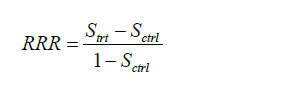
where Strt is the survival probability in the treated group and Sctrl is the survival probability in the control group. The code for the calculation is as follows:

The result is shown in Figure 1. It is noteworthy that there is a large difference between RD and RRR at the beginning.

Bootstrap methods for computing confidence intervals
Bootstrap methods are widely used for the estimation of the confidence interval for quantities of interest (7,8). The method is to draw random samples with replacement from the original sample, so that each of the new samples is of the same size as the original sample. The quantities of RD and NNT can be estimated from each bootstrap sample. The large number of bootstrap samples allows an equal number of RDs to be estimated. The bootstrap 95% confidence interval will be the 2.5th and 97.5th percentiles of RDs across the bootstrap samples (9). Before running the bootstrap procedure, we need to define a function to calculate the RD and NNT.

The rdnnt function receives three parameters which are data, i and time. The data is the original sample and the index i allows the function boot to select samples. The time points at which RD and NNT are estimated are defined by the time argument. There is also an optional parameter frm that gets passed to cph as its formula parameter, which allows us to re-use this function with other datasets whose variables have different names and/or models with different choices of terms. The cat('.') function makes a line of dots to grow on the screen, one for each iteration, so the user doesn't think it freezes. The computation process is based on the Austin method and the code is the same as having been described above. The bootstrap procedure can be run with the following code.

In the boot() function (package boot v1.3-18), the data is the original data frame with each row representing one multivariate observation; statistic is a function that, when applied to data, returns a vector containing the statistic(s) of interest. R is the number of bootstrap replicates; time is an argument passed to the statistic function. The bootstrap procedure may take a long time. The returned value is a list of objects. For example, the object t0 returns the estimated value of RD and NNT when applied to data, while the object t is a matrix with 1,000 rows, one for each bootstrap replicate, with the result of calling the function statistic on the bootstrapped replicates.

The above code creates a data frame containing RD and NNT, and relevant confidence intervals. The first line generates two objects for the placeholder for the confidence intervals of RD and NNT. The for loop calculates bootstrap confidence intervals through follow-up time points. The core function in the for loop is the boot.ci() function. It receives an object returned by the boot() function. Here, it is the results object. The type argument specifies the type of intervals required. “bca” dictates that the intervals are calculated using the adjusted bootstrap percentile (BCa) method. The index argument specifies the position of the variable of interest in results$t0. Finally, the rdci and nntci are combined into an object named tabci. Then we put all quantities into a data frame and rename the columns.

The above output shows the RD and NNT, as well as their confidence intervals. The time is a variable containing the selected time points for RD and NNT calculation. “rd” is the column name for RDs. “rdl” and “rdu” are lower and upper limits of the 95% confidence intervals. “nnt” is the column name for NNT. “nntl” and “nntu” are lower and upper limits of the 95% confidence intervals for NNT. The following code draws a plot showing RD and NNT across analysis time.

The result is shown in Figure 2. It appears that the RD decreases and the NNT increases over time. The left axis is in RD scale, whereas the right axis is in NNT scale. The par(new=T) dictates that the next high-level plotting command will not clean the frame before drawing as if it were on a new device. It is a trick to plot another y-axis with a different scale.

Pseudo-value model to estimate RD
Survival analysis has been developed as an independent area in statistics because it encompasses incomplete follow-up data (e.g., censored data). Without such incomplete data, survival times of all subjects are known and conventional regression model could be used for the survival time. With censored data, the survival time needs to be modelled in special forms such as the Cox model or accelerated failure time model. An alternative to the conventional survival analyses is to use pseudo-values. More mathematical details underlying pseudo-value in survival analysis can be found in references (10,11). This article focuses on how to estimate RD and NNT using R code with the pseudo-value model. The first step is to compute pseudo-observations at given time points for each subjects (12).

The pseudo package (v1.1) is employed to build pseudo-value model (13). The cutoffs object is a vector that stores time points at which pseudo-values are to be computed. The pseudosurv() function requires follow up time (time), status indicator (event) and a vector of time points at which pseudo-values are to be computed (tmax). The returned object is a list containing two objects time and pseudo. time contains the ordered time points at which pseudo-values are to be computed, while pseudo is a matrix with each row representing an individual and each column representing a time point. Before fitting a generalized estimating equation (GEE), we need to reshape the dataset.

The above output shows that the reshaped original dataset where each subject is expanded to several rows, with each row representing a time point. The pseudo-values at a given time point for each subject are shown in the pseudo column and the time points are shown in the tpseudo column. If there was no censoring, the pseudo-value for a subject at a given time would be 1 if he or she was alive at that time, and 0 otherwise. In the presence of censoring, the values are adjusted, but very close to 1 or 0 depending on the vital status of the patient.

GEE model is fit with the geepack package (v1.2-1) (14). By specifying the identity link function in the GEE model, the estimated coefficient is the RD for binary covariates (15). In the example, the coefficient of x (0.33) is the RD between treated and control groups, assuming that RD is time consistent. However, such an assumption could not literally be true and we need to include an interaction term between time and x.

Note there is an interaction between time and x being specified in the GEE model. The time is transformed by the restricted cubic spline function (16). The results are very close to that estimated using the Austin method.

The result shows that the RDs estimated by the Austin method is greater than that estimated by pseudo-value method, but they are close to each other (Figure 3).

Altman’s methods when there is no individual level data
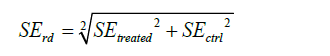
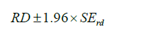
Altman and colleagues proposed that if the standard errors (SEs) of the survival probabilities of the treated and control group were given, SE of RD could be estimated using the equation (17):
then the 95% confidence interval of RD can be estimated as:
In R, the computation can be done with the following code.

However, the confidence intervals after the fifth time point span 0, which are quite different from that obtained with the bootstrap method. Possibly, the Altman’s method is used when there is no individual-level data and thus the results may not be comparable to other estimators.
Summary
The article provides a step-by-step tutorial on the computation of RD and NNT in survival analysis. An artificial dataset containing survival data was employed to illustrate the computation with R. Several methods exist to estimate RD and NNT: the Austin’s method, Altman’s method and pseudo-value procedure. The Altman’s method is used when there is no individual-level data and thus the results may not be comparable to other estimators. The confidence interval can be estimated using bootstrap technique. As compared with RRR, RD or NNT provides more complete information on the risks and benefits of an intervention. In research practice, the rule of thumb is to report both RRR and RD to make the evidence more informative for clinicians and other workers involved in guideline development.
Acknowledgements
Funding: The study was supported by Zhejiang Provincial Natural Science foundation of China (LGF18H150005).
Footnote
Conflicts of Interest: The authors have no conflicts of interest to declare.
References
- Fisher LD, Lin DY. Time-dependent covariates in the Cox proportional-hazards regression model. Annu Rev Public Health 1999;20:145-57. [Crossref] [PubMed]
- Hernán MA. The hazards of hazard ratios. Epidemiology 2010;21:13-5. [Crossref] [PubMed]
- Coory M, Lamb KE, Sorich M. Risk-difference curves can be used to communicate time-dependent effects of adjuvant therapies for early stage cancer. J Clin Epidemiol 2014;67:966-72. [Crossref] [PubMed]
- Moriña D, Navarro A. Competing risks simulation with the survsim R package. Communications in Statistics - Simulation and Computation 2016;8:1-11.
- Austin PC. Absolute risk reductions and numbers needed to treat can be obtained from adjusted survival models for time-to-event outcomes. J Clin Epidemiol 2010;63:46-55. [Crossref] [PubMed]
- Harrell FE. rms: Regression Modeling Strategies. Available online: https://CRAN.R-project.org/package=rms, 2018.
- Efficient bootstrap computations. In: Efron B, Tibshirani RJ. editors. An Introduction to the Bootstrap. Boston, MA: Springer US, 1993:338-57.
- Davison AC, Hinkley DV. Bootstrap Methods and Their Applications. Cambridge: Cambridge University Press, 1997.
- Doğan CD. Applying bootstrap resampling to compute confidence intervals for various statistics with R. Eurasian Journal of Educational Research 2017;17:1-18. [Crossref]
- Andersen PK, Perme MP. Pseudo-observations in survival analysis. Stat Methods Med Res 2010;19:71-99. [Crossref] [PubMed]
- Parner ET, Andersen PK. Regression analysis of censored data using pseudo-observations. Stata Journal 2010;10:408-22.
- Klein JP, Gerster M, Andersen PK, et al. SAS and R functions to compute pseudo-values for censored data regression. Comput Methods Programs Biomed 2008;89:289-300. [Crossref] [PubMed]
- Perme MP, Gerster M. pseudo: Computes Pseudo-Observations for Modeling. 1st ed. Available online: https://CRAN.R-project.org/package=pseudo, 2017.
- Halekoh U, Højsgaard S, Yan J. The R Package geepack for Generalized Estimating Equations. Journal of Statistical Software 2006;15:1-11. [Crossref]
- Ambrogi F, Biganzoli E, Boracchi P. Model-based estimation of measures of association for time-to-event outcomes. BMC Med Res Methodol 2014;14:97. [Crossref] [PubMed]
- Herndon JE 2nd, Harrell FE Jr. The restricted cubic spline as baseline hazard in the proportional hazards model with step function time-dependent covariables. Stat Med 1995;14:2119-29. [Crossref] [PubMed]
- Altman DG, Andersen PK. Calculating the number needed to treat for trials where the outcome is time to an event. BMJ 1999;319:1492-5. [Crossref] [PubMed]

