
Exploring heterogeneity in clinical trials with latent class analysis
Introduction
RCTs, as the gold standard trials, applicable into the assessment of effectiveness of treatments in clinic routines, aim to reduce the bias affected by confounding factors by means of double blind and randomization assignments design, so that the accuracy of assessment could be improved and the effectiveness of drugs could be interpreted more objectively. However, the quality of a clinical trial is often compromised by case mix or heterogeneity of the study population. Typically, the patient inclusionary and exclusionary criteria include clinically observed indicators such as the diagnosis, stage of disease, age (categorized into age groups), gender, medical history, and comorbidities. Although every effort has been made to purify the study population that the biological efficacy can be fully exploited (1), the heterogeneity induced by unmeasurable factors such as genomics and socioeconomic status (e.g., occupation, income, and education) cannot be fully addressed. As a result, even the most carefully selected patient population can exhibit remarkable heterogeneity in clinical trials. Thus, meaningful subgroups of patients based on endorsed response patterns need to be identified to maximize the beneficial effects of a given intervention. For example, the study population in a clinical trial may comprise of two sub-phenotypes wherein the studied effective intervention may benefit one sub-phenotype however not benefit or harm the other sub-phenotype. Additionally, the subgroups of patients may differ in the course, prognosis, and even comorbidity patterns of the disease/disorder of interest for a clinical trial; such information may also create differential effects for the assessed intervention.
Acute respiratory distress syndrome (ARDS) is a common disease in the intensive care unit and it can be diagnosed in the presence of hypoxia induced by bilateral lung inflammation. Although patients with ARDS have long been considered as a study population in clinical trials, this group of patients actually encompasses a heterogeneous population. Investigators have successfully identified sub-phenotypes of ARDS by using inflammatory biomarkers, and the results showed that these sub-phenotypes responded differently to fluid therapy (2,3).
Typically, subgroup analysis performed in clinical trials divides study population by one or two factors. For example, patients can be categorized into subgroups with or without diabetes. The complex relationship (e.g., interactions, higher-order intersections and etc.) between manifest (observed) variables cannot be adequately explored with conventional subgroup analysis. In situations when there are, for example, 6 manifest variables and each has 2 response levels, there will be a total of 26=64 possible response patterns. However, some of the response patterns may only be present in a handful of patients, or even not exist in the real-world setting (4).
A popular method to address patient heterogeneity is finite mixture models, which is a statistically sophisticated framework for identifying meaningful subgroups of patients that are not directly observable. Latent class analysis (LCA) and latent profile analysis (LPA) are special forms of the finite mixture models; which allows us to identify a finite number of latent subgroups and to explore how treatment effect varies across these subgroups (5). The former assesses categorical symptom indicators while the latter assesses continuous indicators for latent group classification (6). Such person-centered approaches transcend limitations imposed by diagnostic categories and classify patients into latent homogenous classes based on similar response patterns (6). Latent subgroups of patients are compared with reference to shape (qualitative differences) symptom levels (quantitative differences) (7). LCA/LPA is more robust and reliable compared to analytically similar cluster analyses because they account for measurement error and use objective criteria to determine the optimal class solution. Identification of such meaningful latent subgroups allows investigators to explore differential treatment effects across these subgroups (8). This article aims to provide a step-by-step tutorial on how to perform LCA in R. In clinical trials, we prefer LCA because continuous variables can be easily converted to categorical variables, but the reverse is not true.
Brief description of LCA
The LCA is based on probabilistic models to create classes or subgroups in a heterogeneous population. This model assumes the existence of unobservable classes which we can measure or observe the consequences or effects.
To describe the latent class model, we adopt the following notations: Let c be the latent class c =1,…,C and v the manifest variable, v=1,…,V. We denote s the response patterns or the outcome vector, s = 1,…,S, where S represents a list of responses. Let s(v) be the response levels of the variable v, s(v)=1,…,Is.
We denote Ps the probability of the outcome vector s which can be written as (9)
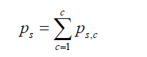
where ps,c denotes the unobserved probabilities of falling simultaneously in the categories defined by vector s and the latent class c. The probability of outcome vector c conditional on latent class c is denoted by ps/c. Assuming conditional independence, ps,c can be written as
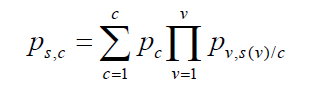
The parameters pc (the size of class) and pv,s(v)/c [probability of category s(v) for variable v conditional on class c] are estimated by using the EM algorithm (10). This algorithm is made up of two important steps: expectation step denoted by E and the likelihood maximization step denoted by M. The first step consists on calculating the expectation of the log-likelihood assuming that we have the information about classes. The second step consists of the maximization of log-likelihood function.
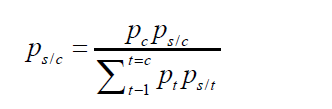
The posterior probabilities that permit to affect individuals to the latent classes is given by:
Dataset simulation
In this tutorial, an artificial dataset is generated by using the poLCA.simdata() function shipped with the poLCA package (11). We first install and load the package.

Then, we proceed to generate a simulated dataset.

The probs object is a list of matrices with dimensions equal to the number of classes (the number of rows) by the number of responses (the number of column). Each matrix corresponds to one manifest variable (from Y1 to Y5), and each row contains the class-conditional outcome probabilities. Note that each row sums to one. For example, the manifest variable Y2 contains two responses and Y4 contains 4 responses. The ability to incorporate polytomous manifest variables is a feature of the poLCA package. Also note that all matrices have the same number of rows because it represents the number of classes. The poLCA.simdata() function generates an artificial dataset. The number of observations is 1000, and the prior class probabilities are 0.2, 0.3 and 0.5 for the three classes.
In many situations, it is of interest to investigate whether the treatment effect varies across latent classes. Thus, we also simulate a variable trt representing the treatment group and an outcome variable representing a binary clinical outcome.

In the second line, a two-level factor variable trt was created with equal size in both levels. The object z is a linear predictor of a logistic regression model. The coefficient of each variable is arbitrarily assigned. The factor variable is converted to a numeric variable by the as.numeric() function. The linear predictor is then converted to probability by logit link function. Then, the outcome variable is generated by assuming a binomial distribution.
To choose the best number of classes
The correct selection of the number of latent classes represents a critical problem because it can significantly affect substantive interpretations (12). Indeed, an incorrect selection of latent classes can lead to an incorrect interpretation of the studied phenomenon. The definition of the number of classes from a population is commonly achieved by using a likelihood ratio test (LMR). This is often used to compare two models (nested models deriving from each other by adding or deleting terms) under the assumption that these two models correctly fit the data. When many models need to be compared, the risk of rejecting the null hypothesis when it is true increases substantially. A number of methods, including information criteria (13), parametric resampling, etc., have been proposed to choose the number of classes. Information criteria including Akaike Information Criterion (AIC) (14), Bayesian Information Criterion (BIC) (15), consistent Akaike Information Criterion (cAIC), adjusted Bayesian Information Criterion (aBIC) (16) are among the most practical methods and require much less computational effort than other methods such as parametric resampling. The AIC is generally valid for the small sample models, though it is not useful for determining the number of classes in general. Other proposed method to judge model fit include Lo-Mendell-Rubin adjusted likelihood ratio test (LMR) (17), Likelihood ratio/deviance statistic, Bootstrap likelihood ratio test (BLRT) (18), and entropy. Typically, several latent class models with various numbers of classes are fit, and their statistics of model fit are compared to choose the best one. Sometimes, the subject-matter knowledge should also be considered when considering the number of classes. Thus, a combination of fit indices (rather than sole reliance on one index), coupled with a consideration of theory and interpretability is recommended to determine the optimal latent class model (8,19). According to the recommended fit indices, the optimal class solution would have the lowest BIC values, lowest aBIC values, a significant LMR value, a significant BLRT p value, relatively higher entropy values, and conceptual and interpretive meaning (8,20,21). When comparing a K-class model with a K-1 class model, a significant LMR test indicates that the model with K classes is optimal (8).
The following loop generates a series of latent class models with one to five classes.

The first line creates a formula in the form of response~predictors. The manifest variables Y1 to Y5 are response variables that characterize the latent class. Note that only non-zero integer variables are allowed, negative or decimal values will return an error message. For continuous variables, users need to convert them into categorical variables. In the formula, no predictor of latent class is added, thus a numeral 1 is added to the right of the “~” symbol. The second line assigned a numeral 5 to k, indicating a maximum of 5 classes will be allowed in the following latent class models. In the for loop, the assign() function is employed to assign a value to a name. The values are a series of objects of the class poLCA, and the object names are different in each loop cycle. The poLCA() is the main function that it estimates latent class models for polytomous outcome variables. The first argument is a formula defined previously. The data argument is a data frame containing variables in the formula. After the loop, five latent class models are created in the environment with the names lc1, lc2, lc3, lc4 and lc5.

The above codes prepare to create a table containing statistics reflecting model fit. The first line creates a data frame with arbitrary values, but there should be 7 columns. Then the column names are assigned to represent the 7 most commonly used model fit statistics.
The entropy-based measures can be a poor tool for model selection, as stated by Collins LM that “Latent class assignment error can increase simply as a function of the number of latent classes, so indices like entropy often decrease as the number of latent classes increases. In other words, class assignment can look better purely by chance in a two-latent-class model than in a comparable model with three or more latent classes.” (22). However, since entropy is widely used in research practice, we illustrate how to compute entropy here. The poLCA.entropy() shipped with the poLCA package is able to calculate entropy when the number of response is the same for all manifest variables. However, when the numbers of response are not equal for all variables, the poLCA.entropy() function will report an error. Thus, we modified the function to incorporate circumstances when the number of response is unequal. In poLCA package, the entropy is defined as (11):

where pc is the share of the probability in the cth cell of the cross-classification table. The function can be rewritten as:

More commonly, the mathematical equation for entropy is given by (23) (https://www.statmodel.com/download/relatinglca.pdf):
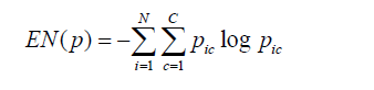
Where pic denotes the estimated posterior probability for individual i in class c. C is the number of classes and N is the number of observations. The entropy equation is bounded from [0,

The “lc$posterior” extracts the posterior probabilities for all observations belonging to a class.

The above code examines the posterior distributions of the first observation in the lc3 model. It appears that this observation is most likely to belong to class 3 (e.g., with a posterior probability of 0.81). Other observations can be examined in the same way.
Relative entropy is a rescaled version of entropy by the following equation (23):
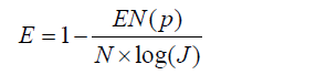
where J is the number of classes. The R function for computation of relative entropy is as follows:

Then we proceed to calculate the model fit statistics for all fitted latent class models.

The poLCA() function automatically calculates all statistics assessing model fit, and we just need to extract them from the returned poLCA objects and put them in a data frame. The last two lines round the returned values to 2 decimal places and remove the first row. Then, a new variable Nclass is added to denote the number of classes. The results can be viewed as follows:

The model fit can also be visualized to facilitate interpretation. First of all, we need to reformat the data frame tab.modfit.

The results2 data frame is a long format that the labels for model fit statistics are formatted in long style. The value column is the values for respective statistics. Then, this data frame can be passed to the ggplot() function (24).

The result is a plot showing the changing values of model fit statistics by varying number of classes (Figure 1). It appears that latent class model with 3 classes has the smallest values in aBIC and cAIC. However, the relative entropy is not optimal with 3 classes (as mentioned above, entropy can be a poor tool for model selection). Although the 5-class model has a greater entropy value than the 3-class model, three of the 5 classes have very low population shares. Collectively, the 3-class model is the optimal model, taking into account of the combination of statistical fit indices, parsimony and interpretative value.


The lca_select() function
The lca_select() function makes it easier to choose the right model based on the information criteria (created by A.A.). In this function, we added more information criteria such as Hurvich and Tsai Criterion (HT) (25), Modified AIC (mAIC) (26), Hannan and Quinn Criteria (HQ) (27), Corrected Akaike Information Criterion (AICc) (28). The function is defined as follows:

Then we proceed to compute and display model fit statistics with the following code.

In the example, the number of classes to be chosen is 8 and the information criteria as well as other statistics is shown in Table 1. Furthermore, the information criteria to choose the number of classes are displayed in Figure 2. It appears that the 3-class model has the lowest values on all information criteria, and it is reasonable to choose the 3-class model.

Full table

Model visualization
The generic function plot() can be applied directly to the poLCA object to visualize the latent class model.

The result is shown in Figure 3. The overall population is divided into 3 classes by the five manifest variables. The graphic presents probabilities of categories s(v) (response value) for variable v conditional on class c. For example, the class 2 is characterized by a large probability of response value 2 in Y2 and 3 in Y5. These characteristics can be interpreted with subject-matter knowledge.

The latent class model can also be visualized in 2D plot.

The Figure 4 gives the same information as that of the Figure 3, but the responses are displayed in 2-D format.

Differential treatment effects across latent classes
The 3-class model is considered as the best fitted model and the 3 classes can be considered as subgroups of the overall study population. The next task is to investigate whether the treatment effects vary across latent classes. As mentioned earlier, we have generated the variable trt and outcome, corresponding to the treatment group and the binary outcome. Lanza ST and colleagues described two methods to examine differential treatment effects (4): (I) a classify-analyze approach involving logistic regression model, and (II) a model-based approach. The classify-analyze approach involves two steps, “classify” step and the “analyze” step. The first step is to obtain the posterior probability of each patient and assign them to the latent class with the maximum probability, which is based on the maximum-probability assignment rule (29,30). Next, the “analyze” step involves building a logistic regression model with the outcome variable as the dependent variable. The treatment and latent class membership are included in an interaction term (31). This is the conventional regression/analysis of variance approach to test differential treatment effects across subgroups. The model-based approach involves multiple group LCA which is not currently implemented in the poLCA package.

The logistic regression model is fitted with generalized linear model (32). The trt and latent class group membership variables are included as an interaction term. The “lc3$predclass” extracts the latent class membership for each individual patient, and it is converted to a factor variable because the class membership values 1, 2 and 3 have no numeric relationship. In the model, class 1 is regarded as the reference class, against which other classes are compared. The result shows that the treatment effect is not significantly different for the class 1 vs. class 2 comparison (β=2.031, SE=0.241, P=0.338), but the effect is significantly different for the class 1 vs. class 2 comparison (β=0.847, SE=0.428, P=0.048). The treatment seems to be more effective in reducing adverse outcome for patients in class 2. For subject-matter audience, it is convenient to transform the regression coefficients to odds ratios. Patients in the class 2 group assigned to treatment group are e0.231−0.847=0.54 times as likely to report outcome 1 compared to the control group. In other words, the treatment results in a 50% risk reduction for patients in class 2.

The first line attaches the class membership variable predclass to the original data frame. Then a data frame containing proportions is generated, which can be passed to the barplot() function. The result shows that the treatment is able to reduce the risk of outcome 1 by nearly 50% (Figure 5), whereas such a beneficial treatment effect is not observed in the other two classes.

Acknowledgements
Funding: The study was supported by Zhejiang provincial natural science foundation of China (LGF18H150005).
Footnote
Conflicts of Interest: The authors have no conflicts of interest to declare.
References
- Nallamothu BK, Hayward RA, Bates ER. Beyond the randomized clinical trial: the role of effectiveness studies in evaluating cardiovascular therapies. Circulation 2008;118:1294-303. [Crossref] [PubMed]
- Calfee CS, Delucchi K, Parsons PE, et al. Subphenotypes in acute respiratory distress syndrome: latent class analysis of data from two randomised controlled trials. Lancet Respir Med 2014;2:611-20. [Crossref] [PubMed]
- Famous KR, Delucchi K, Ware LB, et al. Acute respiratory distress syndrome subphenotypes respond differently to randomized fluid management strategy. Am J Respir Crit Care Med 2017;195:331-8. [PubMed]
- Lanza ST, Rhoades BL. Latent class analysis: an alternative perspective on subgroup analysis in prevention and treatment. Prev Sci 2013;14:157-68. [Crossref] [PubMed]
- Rindskopf D, Rindskopf W. The value of latent class analysis in medical diagnosis. Stat Med 1986;5:21-7. [Crossref] [PubMed]
- McCutcheon A. Latent Class Analysis. Newbury Park, CA: SAGE Publications, 1987.
- Nugent NR, Koenen KC, Bradley B. Heterogeneity of posttraumatic stress symptoms in a highly traumatized low income, urban, African American sample. J Psychiatr Res 2012;46:1576-83. [Crossref] [PubMed]
- Nylund KL, Asparouhov T, Muthén BO. Deciding on the number of classes in latent class analysis and growth mixture modeling: a monte carlo simulation study. Struct Equ Modeling 2007;14:535-69. [Crossref]
- Mooijaart A, van der Heijden PG. The EM algorithm for latent class analysis with equality constraints. Psychometrika 1992;57:261-9. [Crossref]
- Dempster AP, Laird NM, Rubin DB. Maximum likelihood from incomplete data via the EM algorithm. Journal of the Royal Statistical Society 1977;39:1-38.
- Linzer DA, Lewis JB. poLCA: An RPackage for Polytomous Variable Latent Class Analysis. Journal of Statistical Software 2011;42:1-29. [Crossref]
- Yang CC. Evaluating latent class analysis models in qualitative phenotype identification. Computational Statistics & Data Analysis 2006;50:1090-104. [Crossref]
- Lin TH, Dayton CM. Model Selection Information Criteria for Non-Nested Latent Class Models. Journal of Educational and Behavioral Statistics 1997;22:249-64. [Crossref]
- Akaike H. Factor analysis and AIC. In: Regression modeling strategies. New York, NY: Springer New York; 1998:371-86.
- Schwarz G. Estimating the Dimension of a Model. The Annals of Statistics 1978;6:461-4. [Crossref]
- Sclove SL. Application of model-selection criteria to some problems in multivariate analysis. Psychometrika 1987;52:333-43. [Crossref]
- Lo Y. Testing the number of components in a normal mixture. Biometrika 2001;88:767-78. [Crossref]
- McLachlan G, Peel D. Finite Mixture Models. Hoboken, NJ, USA: John Wiley & Sons, Inc., 2005.
- Tein JY, Coxe S, Cham H. Statistical power to detect the correct number of classes in latent profile analysis. Struct Equ Modeling 2013;20:640-57. [Crossref] [PubMed]
- Nylund K, Bellmore A, Nishina A, et al. Subtypes, severity, and structural stability of peer victimization: what does latent class analysis say? Child Dev 2007;78:1706-22. [Crossref] [PubMed]
- DiStefano C, Kamphaus RW. Investigating Subtypes of Child Development. Educational and Psychological Measurement 2016;66:778-94. [Crossref]
- Collins LM, Lanza ST. Latent class and latent transition analysis: with applications in the social, behavioral, and health sciences. In: Lanza ST. editor. Latent class and latent transition analysis: with applications in the social, behavioral, and health sciences (wiley series in probability and statistics). Hoboken, NJ: John Wiley & Sons, Inc., 2010:295.
- Jedidi K, Ramaswamy V, Desarbo WS. A maximum likelihood method for latent class regression involving a censored dependent variable. Psychometrika 1993;58:375-94. [Crossref]
- Ito K, Murphy D. Application of ggplot2 to Pharmacometric Graphics. CPT Pharmacometrics Syst Pharmacol 2013;2:e79-16. [Crossref] [PubMed]
- Hurvich CM, Tsai CL. Regression and time series model selection in small samples. Biometrika 1989;76:297-307. [Crossref]
- Andrews RL, Currim IS. A comparison of segment retention criteria for finite mixture logit models. Journal of Marketing Research 2003;40:235-43. [Crossref]
- Hannan EJ, Quinn BG. The Determination of the Order of an Autoregression. Journal of the Royal Statistical Society 1979;41:190-5.
- Sugiura N. Further analysts of the data by akaike' s information criterion and the finite corrections. Communications in Statistics - Theory and Methods 2007;7:13-26. [Crossref]
- Goodman LA. On the Assignment of Individuals to Latent Classes. Sociological Methodology 2016;37:1-22. [Crossref]
- Bakk Z, Tekle FB, Vermunt JK. Estimating the Association between Latent Class Membership and External Variables Using Bias-adjusted Three-step Approaches. Sociological Methodology 2013;43:272-311. [Crossref]
- Bray BC, Lanza ST, Tan X. Eliminating Bias in Classify-Analyze Approaches for Latent Class Analysis. Struct Equ Modeling 2015;22:1-11. [Crossref] [PubMed]
- Zhang Z. Model building strategy for logistic regression: purposeful selection. Ann Transl Med 2016;4:111-1. [Crossref] [PubMed]

