
Time-varying covariates and coefficients in Cox regression models
Introduction
Time-varying covariance occurs when a given covariate changes over time during the follow-up period, which is a common phenomenon in clinical research. For example, in a patient with sepsis, the C-reactive protein (CRP) may be measured repeatedly to evaluate inflammatory status until it returns normal (1). In clinical oncology, the recurrence status of a patient is usually checked at a predefined time interval. In many cases when studying the relation between a survival outcome and covariate(s), investigators will only consider the baseline value of the covariate, which however, fails to consider the relation of the survival outcome as a function of the change of the covariate. For example, the effect of smoking on cancer risk has been extensively studied. However, the smoking status is ever changing during the follow up period (2). Such a covariate can be considered as a time-varying covariate.
Time-varying covariates can be classified as either internal, when the path is affected by survival status, or external, when the covariate is the fixed/defined covariate (3). An internal covariate is typically the output of a stochastic process generated by an individual under study and observed only as long as the subject survives and uncensored. Thus, such data are found in clinical trials where records of patients’ general condition are made at regular intervals and where failure time occurs when the patient dies.
An external covariate X(⋅), in contrast, may influence the rate of failure over time, but its path up to time t > v is not affected by the occurrence of failure time at time v. It is also a derived or predetermined covariate. Examples of external covariates are age of an individual in a trial of long duration, or a measure of airborne pollution as a predictor of the frequency of asthma attacks. The covariate allows incorporation of a time interaction function X(t) or X(g(t)) (4,5). Consider the general hazard model for failure time proposed by Cox [1972] (6),
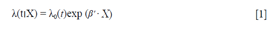
where λ0(t) is the baseline hazard function (possibly non-distributional) and β' = (β1, β2, .., βp) is a vector of regression coefficients. In the simple form of the Cox model, X is a vector of time-fixed covariates.
One approach for using time-varying covariate data is to extend the Cox proportional hazard model to allow time-varying covariates (7).

where β' and γ' are coefficients of time-fixed and time-varying covariate respectively. Suppose we let Z(t) represent the covariate, then

and the hazard ratio is
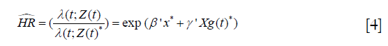
which is a non-constant hazard rate. Such functionality can be implemented in many sophisticated software and here we will illustrate how to perform such kind of analysis with R-program (8). The main approaches for survival analysis with time-varying covariates are time-dependent Cox models (7) and the joint modeling of longitudinal and survival data (9). Time-dependent Cox models are more appropriate for external covariates (e.g., external covariates vary as a function of time, independent of the failure time) and are considered in this paper.
In a slightly comparable situation, a covariate is measured at baseline but its effect on the outcome is not constant over the follow-up time, which is a violation of the proportional hazards assumption (7). In that case a time-varying coefficient can be incorporated into the Cox regression model to fit such kind of data. In fact, to check the proportional hazards assumption after fitting a Cox regression model is the same as identifying time-varying coefficients. In this paper, we will also show how to check the proportional hazards assumption after fitting a Cox regression model, and in case there is a violation to the assumption, show how the model should be modified to best describe the data.
In fact, if the time-varying coefficient can be written as g(β,t) = βg(t), the model with a time-varying coefficient can be expressed as a model with time-varying covariate with a constant coefficient (10). The hazard of failure is related to the covariate by the equation:

where β is a coefficient related to the covariate X and g(β, t) is a specific function of time that can be defined by investigators. If g(β, t) is a simple function, it can be written as g(β, t) = βg(t). Then the hazard function can be written as:

where X(t)= g(t)X. This equation shows that a time-varying coefficient (g(β, t)) model can be modelled with a set of time-varying covariates (X(t)) (10).
Verification of proportionality assumption can be done by any of the two known approaches, graphical visualization and numerical approaches. Later in this work we look at Schoenfeld residual scaled plot and log(-log(S(t))) plot. For each predictor in the model, Schoenfeld residual are defined and the residuals for the predictors are plotted against the ranked/transformed failure time.
Working example on time-varying covariates
To show how to estimate a survival model with time-varying covariates we will construct a simulated dataset. To show how to combine such data we will therefore simulate two data frames in R, one containing the baseline covariates (age and group) and the other a time-varying covariate. With the package survsim (11), a dataset of 100 patients involving continuous and categorical covariates, and a time-to-event outcome can be generated. The simulated dataset is for illustration purpose only and there is no clinical relevance.

The above code generates a data frame containing two time-fixed variables named “grp” (abbreviated from group) and “age”. The age variable is assumed to be normally distributed with the mean=70 and standard deviation of 13. The grp variable is a factor (categorical or binary) variable with two levels 0 and 1. The status variable is the outcome status at the corresponding time point. The start and stop variables define the start and stop time points of a follow-up interval for each individual. The underlying mechanisms of the data generation is beyond the scope of this paper, but interested readers can consult the R document by typing “?simple.surv.sim”. Alternatively, survival times with time-varying covariates can be generated following the methods proposed by Austin (12).
Next, we generate a data frame in a counting process data structure (13), in which each individual is represented by one or more rows. In such a data frame, each row represents a follow up time interval at which the value of a covariate is recorded. The following code generates a time-varying covariate named crp (C-reactive protein) which is assumed to have a normal distribution with a mean of 100 and a standard deviation of 40. In reality, the crp value may be skewed. Although a simple binary covariate such as transplantation, surgery or starting of medication, could be good for demonstrating, we incorporate a numeric variable because such kind of variables are common in reality.

The number of follow up time intervals is randomly generated for each subject with a maximum of 10. With a for loop function, crp values are assigned to each follow up time interval. A variable id is generated in the for loop, which is a tag for identification of a distinct subject. Finally, a data frame named df.td containing a time-varying covariate crp is generated.
Merging data frames with tmerge() function
Data containing information on time-varying covariates is often stored in different format than what is required by statistical programs. The first step in analyzing time-varying covariates in survival analysis is to reshape the data frame so that there are multiple rows (time intervals) for each subject, along with covariate values that apply across these intervals. Such a format is also known as the counting process style or (start, stop) form of data. The survival package provides a good function tmerge() for this purpose (7,14). The function usually runs in multiple passes, with the first run defining the basic structure and subsequent runs add variables to that structure. This run does not change the values of original variables but it defines the basic structure of the df object, which is essential for subsequent steps.

In the new data frame df, several variables are added including tstart and tstop representing the start and stop of the follow up interval. The variable endpt is the same as the variable status indicating whether the event is observed. The variable z is the individual heterogeneity generated in the simple.surv.sim() function according to the specified distribution. The value of z is 1 for most observations because the use of the round() function. Next, the total follow-up time is split into the simulated time intervals from dataframe df.td and these intervals are censored by the total follow-up time.

The first argument of tmerge() function is the primary dataset to which new covariates will be added. The second argument is another dataset that contains new covariates. The “newname=tdc(y,x)” argument creates a new time-varying covariate. The argument y is on the scale of start and stop time. The second argument x is not mandatory. If x is missing the count variable starts at 0 for each subject and becomes 1 at the time of the event. In case x is present the count is set to the value of x. In the example, a crp value is added at each interval. The updated data frame df is in the counting process style that each subject can take several rows. For example, subject 2 has 6 rows, and crp values are different at each row. However, the values of time-fixed variables such as age and grp are consistent within each subject.
Fitting the Cox model with a time-varying covariate
Next, we will model the survival times as a function of group, age and crp values with Cox regression:

With the reshaped dataset, the fitting of Cox regression model is straightforward. The output of the coxph() function shows that there is only one hazard ratio (exp(coef)) for the variable crp, which is similar for the two time-fixed covariates age and grp. In the Cox regression model with time-varying covariates, the follow-up time of each subject is divided into shorter time intervals. However, we do not have to take into account in the analysis that individuals may have multiple rows unless there are multiple events per individual. The likelihood equations use information on only at most one row per an individual at any time point, since the time intervals of an individual do not overlap (7).
Time-varying coefficients
As noted above, time-varying effect emerges when the proportional hazards assumption is not fulfilled. So, to identify time-varying coefficients is actually to test the proportional hazards assumption after fitting a Cox proportional hazard model. The examination of proportional hazards assumption can be performed using the cox.zph() function shipped with the survival package (14). Below, the lung dataset available from the package survival is employed to illustrate how to explore the proportional assumption.

First, a Cox proportional model is fit by using the coxph() function. The left side of the formula is the response variable defined by the Surv() function with the follow-up time and status for each patient. The right side displays covariates age (in years), ph.karno (Karnofsky performance score rated by physician) and sex (male =1; female =2). The data argument defines the data frame that contains the data with the variables from the formula. The cox.zph() function is the core to the investigation of proportional hazards assumption. The first argument of the function is an object returned by coxph() function.
The output of the function is a table in matrix format with each row representing one variable and the last row is the Schoenfeld’s global test for the violation of proportional assumption (15). Columns of the matrix from left to right show the correlation coefficient between transformed survival time and the scaled Schoenfeld residuals (rho), a chi-square statistic (chisq), and the two-sided P value (p). There is no appropriate correlation for the global test, so an NA is entered in the rho column. The result shows that there is significant deviation from the proportional hazards assumption for the variable ph.karno (P=0.00409). The result can be visualized with generic plot() function. In general, an associated global significant test gives a P value (0.00911) which is an indication of lack of fit of the model.

Figure 1 shows the time-varying coefficient for the variable ph.karno. Note that the time axis is not in linear scale because we used “km” transformation for the time. So in this example we have identified a time-varying coefficients as there appears to be two turning points approximately at values of 180 (the point where the slope of the beta reverses) and 350 (the point where the hazard of the coefficient exceeds the reference for null effect), at which the analysis time can be divided.

Step function to explore time-varying coefficient
One way to model time-varying coefficients is to use a step function, e.g., (g(t) = I(t ≥ to)), where to is a specified value. The idea of this method is to split the analysis time into several intervals and Cox proportional model is stratified for these time intervals. The effect of fixed baseline covariates becomes stronger or weaker over time, which can be explored via stratification by time. As illustrated in Figure 2, the effect of the baseline risk factor ph_karno varies over time, resulting in a series of HRs. With the survSplit() function one can split each record into subrecords at prespecified cut time points in the counting process style as we have seen before.


The first argument of the survSplit() function is a model formula where the model of the survival data can be specified as we have seen before. The cut argument is a vector of cutoff time points. In the example, we cut the analysis time at 180 and 350. The episode option defines a new variable name that will appear in the new data frame. Here, it is “tgroup”. The resulting data frame is in a counting process form so that each subject is split and takes several rows. For example, patient 2 takes three rows. The original row of (0, 455] with a cut vector of (180, 350) will be split into intervals of (0, 180], (180, 350] and (350, 455]. The newly defined variable tgroup identifies which interval each row belongs to. To explain, tgroup=1 identifies the first time interval (0, 180], and tgroup=2 identifies the second time interval (180, 350].

Now the Cox regression model is fit as usual, except that it is stratified by the tgroup variable. From the output, it appears that the variable ph.karno only has a significant effect in the first time interval (tgroup=1). The corresponding HR was 0.97 (P=0.00028). The effects of ph.karno on the remaining two time-windows are not statistically significant. Next, we can take a look at the proportional hazards assumption of this stratified Cox regression model.

The result shows now that there is no correlation between transformed survival time and the scaled Schoenfeld residuals, indicating that the proportional hazards assumption is not violated with the stratified analysis, and judging by the global p-value, the model is fit.
Continuous function to describe the time-varying coefficient
An alternative method to describe the time-varying coefficient is with a parametric continuous function that is specified by the user. Here we illustrate how to perform such an analysis.

In the coxph() function, there is a tt argument to specify the specific transformation of time. In our example, the tt function is defined as “tt = function(x, t, ..) x * log(t+20)”, where x is a fixed covariate with time-varying effect, and t is the analysis time. The tt() function is applied to the variable ph.karno in the model formula as “tt(ph.karno)”. The outcomes of the analysis are:

Both the coefficients for ph.karno and tt(ph.karno) are statistically significant, implying that the effect of ph.karno varies with time. The time-varying effect of ph.karno can be written as β(t) = −0.098+0.015×log(t + 20). We can add a line to the cox.zph plot of the time-varying effect of ph.karno on survival by using the abline() function.

The result is shown in Figure 3. The slope of the red line is 0.015, which is significantly different from the horizontal line (slope=0). The black line shows the time-varying coefficient for the variable ph.karno.

Investigating time-varying coefficient with timereg package
The timecox() function shipped with the timereg package (16) is able to fit a Cox model with both time-fixed and time-varying coefficients. In this case the time-varying effect is tested by resampling method (17). Specification of the models is similar to the way it is done in the survival package.

Cox regression model is fit similarly as in the survival package with the only difference that resampling methods are used for the statistical inference and therefore, the number of simulations has to be specified (n.sim=500). The max.time argument specifies the end of observation period where estimates are computed. The returned results are shown below:

Test for time invariant effects

The first table of the output shows the results of the test for non-significant effect (e.g., the null hypothesis states that the coefficients under test are not significantly different from 0), which shows that both sex and ph.karno have significant effect on survival outcome (P=0.002 and <0.001). The second table shows the test for the time invariant effect. Both the Kolmogorov-Smirnov test and the Cramer von Mises test are used for testing time invariant effects. It appears that the effect of ph.karno is not time-fixed. The effects of all variables over time are visualized in Figure 4.


It is noted from Figure 4 that the effect of ph.karno is steep at the beginning and then flattens out after approximately 180. The variable age has no significant effect because the confidence interval intersects with the null effect reference line. The variable sex has significant effect but the null hypothesis of time invariance effect cannot be rejected. Therefore, we will proceed to set sex and age as time-fixed effect variables by fixing them with the const() function.

The const() function applied to the covariates age and sex specifies them to have constant effects. The age and sex have constant effects of 0.0135 and −0.6210, respectively.
Discussion
When time-varying covariates or coefficients are present, an analyst should consider taking them into account in survival modeling in order to improve the estimation. In this paper, we presented some ways to do this using the R-program. Time-varying covariate was handled with a time-dependent Cox model and time-varying coefficient was described using a step function and a continuous function.
In this article, we only presented some methods dealing with time-varying covariates or coefficients, but other approaches are available. Sometimes the model fit may also be improved by using derived variables from longitudinal measurements. For example, averages of the most recent and all the previous measurements may be used to better describe the cumulative nature of the time-varying covariate or differences of the latest two measurements to model the effects of changes (18). Also the standard deviation of the longitudinal measurements (19) and lagged observations (20) has been used.
With internal time-varying covariates, one could also consider using joint modeling of longitudinal and survival data (9) which was not presented in this article. The idea is to assign a model for a continuously changing covariate which is measured longitudinally in time and possibly with error. This longitudinal model is related to survival times by modeling the joint distribution of longitudinal and survival data. Recent developments and issues in this topic are considered by, e.g., Hickey et al. (21).
Acknowledgements
Funding: The study was supported by Zhejiang Provincial Natural Science foundation of China (LGF18H150005).
Footnote
Conflicts of Interest: The authors have no conflicts of interest to declare.
References
- Zhang Z, Smischney NJ, Zhang H, et al. AME evidence series 001-The Society for Translational Medicine: clinical practice guidelines for diagnosis and early identification of sepsis in the hospital. J Thorac Dis 2016;8:2654-65. [Crossref] [PubMed]
- Pinsky PF, Zhu CS, Kramer BS. Lung cancer risk by years since quitting in 30+ pack year smokers. J Med Screen 2015;22:151-7. [Crossref] [PubMed]
- Collett D. Modelling Survival Data in Medical Research. 3rd ed. Boca Raton: Chapman and Hall/CRC, 2014.
- Adeleke KA, Abiodun AA, Ipinyomi RA. Semi-parametric non-proportional hazard model with time varying covariate. Womens Health Journal 2015;14:68-87.
- Kalbfleisch JD, Prentice RL. The Statistical Analysis of Failure Time Data. Hoboken, NJ, USA: John Wiley & Sons, Inc., 2002.
- Cox DR. Regression Models and Life-Tables. J R Statist Soc B 1972;34:187-220.
- Therneau TM, Grambsch PM. Modeling Survival Data: Extending the Cox Model. New York, NY: Springer New York, 2000.
- R Core Team. R: A language and environment for statistical computing [Internet]. 2017 [cited 2018 Jan 8]. Available online: https://www.R-project.org/
- Henderson R, Diggle P, Dobson A. Joint modelling of longitudinal measurements and event time data. Biostatistics 2000;1:465-80. [Crossref] [PubMed]
- Thomas L, Reyes EM. Tutorial: Survival Estimation for Cox Regression Models with Time-Varying Coefficients Using SASand R. Journal of Statistical Software 2014;61:1-23. [Crossref]
- Moriña D, Navarro A. Competing risks simulation with the survsim R package. Communications in Statistics - Simulation and Computation 2016;8:1-11.
- Austin PC. Generating survival times to simulate Cox proportional hazards models with time-varying covariates. Stat Med 2012;31:3946-58. [Crossref] [PubMed]
- Andersen PK, Perme MP. Pseudo-observations in survival analysis. Stat Methods Med Res 2010;19:71-99. [Crossref] [PubMed]
- Therneau TM. A Package for Survival Analysis in S. version 2.38. CRAN.R-project.orgpackagesurvival. 2015.
- Grambsch PM, Therneau TM. Proportional hazards tests and diagnostics based on weighted residuals. Biometrika 1994;81:515-26. [Crossref]
- Martinussen T, Scheike TH. Dynamic Regression Models for Survival Data. Springer-Verlag New York, 2006.
- Tian L, Zucker D, Wei LJ. On the Cox Model With Time-Varying Regression Coefficients. Harvard University Biostatistics Working Paper 2005;100:172-83.
- Reinikainen J, Laatikainen T, Karvanen J, et al. Lifetime cumulative risk factors predict cardiovascular disease mortality in a 50-year follow-up study in Finland. Int J Epidemiol 2015;44:108-16. [Crossref] [PubMed]
- Muntner P, Shimbo D, Tonelli M, et al. The relationship between visit-to-visit variability in systolic blood pressure and all-cause mortality in the general population: findings from NHANES III, 1988 to 1994. Hypertension 2011;57:160-6. [Crossref] [PubMed]
- Hanson TE, Branscum AJ, Johnson WO. Predictive comparison of joint longitudinal-survival modeling: a case study illustrating competing approaches. Lifetime Data Anal 2011;17:3-28. [Crossref] [PubMed]
- Hickey GL, Philipson P, Jorgensen A, et al. Joint modelling of time-to-event and multivariate longitudinal outcomes: recent developments and issues. BMC Med Res Methodol 2016;16:117. [Crossref] [PubMed]

