
Quality comparision of Flos Lonicerae Japonicae by several dissimilarity methods
Abstract: Computing similarity is extremely important in modern scientific research such as computational biology and data mining. In this paper, we put forward the concept of quantitative dissimilarity (QDS) and define a series of formulations to measure how similar or dissimilar between two objects are in quality and content for their n-dimentional properties, which is based on a simple mathematical model. Through establishing the HPLC fingerprints (HPLC-FPs) of Flos Lonicerae Japonicae (FLJ) to obtain n-dimentional vectors, in which each peak area serves as an element, the authentical quality control of FLJ were successfully implemented by several QDSs. The presented dissimilarity methods can accurately and quantitatively assess all objects differences in n-dimentional properties.
Key words: Quality comparision; Flos Lonicerae Japonicae; quantitative dissimilarity
Introduction
The similarity phenomenon existing universally in nature, science, society and other fields has been playing a great role in evaluating the difference among things. Aristotle, the Greek philosopher, thought “In philosophy, it is usually correct to think over the similarities, although they are far away from each other”. Planck, the German physicist, said “On the surface the images of the nature vary greatly, but the similar simple principle often exists in incoherent fields”. When humans face the world, looking for similarities is their instincts, and they always understand the world through the similarities between the objects. In 1869, Mendeleev, the Russian chemist, had successfully discovered periodic law of elements by studying on the similarities between atomic weights and chemical properties of the elements; and computing similarity plays a more significant role in modern scientific research, such as the diversity and distribution proportion of biological genes or proteins, chemical composition and content distribution of plant medicines, popular ranking of universities.
In ancient study on similarity, people depended mainly on experience and expertise. However, with the development of science and technology, the requirement of the research becomes higher and higher, so that it is hard to precisely measure similarity depending only on experience and expertise. Therefore mathematical tools gradually were introduced into research to give rise to the multivariate data analysis. Such by means of vectors in n-dimension space to study the similarity degrees between objects is called similarity science that mainly contains qualitative similarity and quantitative similarity. Qualitative similarity merely lays stress on the “quality” of the objects, and quantitative similarity investigates their similarity degrees in respect of “quantity”, so they are unified and mutual complementarity. Qualitative similarity adequate is the premise to assessing the quantitative similarity, for quantitative similarity is blind and meaningless without an adequately qualitative similarity; also quantitative similarity would make qualitative similarity more accurate and scientific in measuring for the multivariable objects. Wherever the universal law followed by the similarity may possess similar form. The approach to such form and its law is also the final goal that quantitative dissimilarity (QDS) efforts to achieve.
The resemblance magnitude can be measured by both similarity and QDS, in which similarity describe how larger of resemblance degree between two objects, and the more alike objects the larger similarity. Usually, similarity is positive and typically within 0 to 1 to indicate various degrees of resemblance, where 0 means that two objects are not similar at all and 1 reflects maximal similarity. Dissimilarity represents how big is the difference degree, in which the opposite to similarity, the more similar the two objects the lower the QDS. Dissimilarity may varies within [0, 1] or from _∞ to ∞. The development of QDS has principally involved three stages: similarity research for binary variable, similarity research for multivariate vectors and similarity research based on fuzzy sets. The variable has two attributes (0 or 1) is called binary variable, whose similarity can be measured by simple matching coefficient (SMC) (1,2) and Jaccard coefficient (3,4). This stage rests on qualitative similarity and still has been applied in information retrieval now. Until 1930s, the objects had turned into multivariate vectors, whose similarity measurements mainly included all kinds of coefficients, such as Tanimoto coefficient (5), cosine coefficient, Pearson’s correlation coefficient (6), Dice coefficient (7), Bray-Curtis coefficient (8), Overlap measure and so on. Nei (9,10) has used Nei coefficient to characterize the genetic similaritiy between individuals when he researched the diversity of genes. Also these methods don’t have pretty quantitative properties. Dissimilarity is generally measured by distances, for example the popular Euclidean distance served as a tool to determine the distance between two vectors, in addition Minkowski distance (11,12), Manhattan distance, Chebyshev distance, Mahalanobis distance, Aitchison distance (13,14), Hamming distance, Bhattacharya’s distance (14), Hausdorff distance (15) and Dimension Root similarity (16), Gowda and Diday’s QDS measure (17), Ichino and Yaguchi’s QDS measure (12), Canberra QDS (18) etc. Although they can quantify in some extent, the visualized and comprehensive percent results of quantitative evaluation cannot be given directly. Since 1965 Zadeh (19) proposed fuzzy set theory, fuzzy mathematics had been widely used and rapid developed, fuzzy similarity became an important tool for comparing two groups or two elements (20-24). Its main idea is establishing fuzzy data according to fuzzy set theory and then evaluating their similarities using various coefficients or distances as mentioned above. Due to late start, this method is far from perfect up to now and is used broadly in image processing and recognition.
This paper presented several dissimilarities through establishing a mathematical model to give the qualitative dissimilarities and QDSs, in which the quality comparision based on HPLC-FPs of FLJs was successfully performed. These methods were also suitable for evaluations of the diversities and distribution proportions of biological genes and proteins, evaluations of chemical composition and contents distributions of herbal medicines and computing the popular ranking of universities.
The dual qualitative similarity (DQLS)
If sample vector (SV) is denoted as  =
=  = (x1,x2,…,xn) and the referential vector (RV) as
  =
=  = (y1,y2,…yn), the cosine of the angle (θ) between them is defined as qualitative similarity (SF), as shown in Eq.[1], which clearly reveals the resemble degree between the coordinates in distribution proportion of numerical magnitude. Unfortunately, it does not possess any quantitative properties, for instance, the SF of
  = [1,2,3,4,5] and
  = [10,20,30,40,50] is 1.0, whereas the content of each element in is 10 times as that in . Furthermore, xi and yi contribute differently to SF, respectively, which suffers from the drawbacks that the larger elements seriously mask the smaller ones. If RV and SV are denoted as
 = [1,1,…,1] and
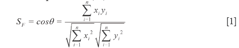
 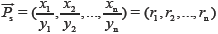 , respectively, then qualitative ratio similarity (SF') is defined by calculating the cosine between and
  , as listed in Eq.[2]. Because of the tendency divided by yi, xi shows equal weights to SF'. However, SF' seriously ignores the contributions of the larger elements to system and overemphasizes those of the smaller elements. Therefore SF and SF' are combined to qualitatively evaluate the similarity between SV and RV and called DQLS, in which they can simultaneously monitor the contributions of both larger elements and smaller elements to system with the characteristics of accuracy and not laying particular stress on any elements. The resemblance of and is judged qualified when SF and SF' no less than 0.9 are servered as the necessary condition to quantitatively evaluate them. Otherwise, it would be meaningless for quantitative similarity evaluations, because the chemicals number attribution and congener content degree does not meet the requirements (25).
The dual quantitative similarity (DQTS)
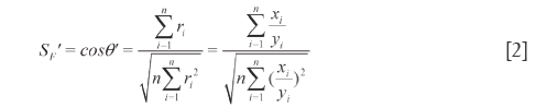
The ratio of module length of to module length of (W) well reflects the relationship of macroscopic content between SV and RV, see Eq.[3], where W is also strongly influenced by the larger elements and subjects to a problem of the smaller elements being masked by the larger ones, either. In addition, θ can also affect W. Apparent content similarity (R) is defined as the sum of the element values of SV divided by that of RV, and its formulation is shown in Eq.[4]. Because of all the elements being summed, the content property of a sample to reference reflected by R is accurate. Nevertheless, in SV, the larger elements and smaller elements may crossly compensate to bring about errors. W and R constitutes the first level dual quantitative similarities (1L-DQTS), which can not only reduce the masking effects of the larger elements in some extent but also equally treat the contributions of the smaller elements to system. Consequently, they are capable of monitoring sensitively the contributions of all elements to the 1L-DQTS (26).
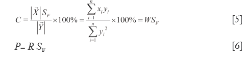
Defined the percentage of projection length of to relative to the module length of as projection content similarity (C), as shown in Eq.[5]. Like W, the larger elements dramatically affect it for they masking the smaller elements. But C is more accurate than W, since it is the ratio of the length of SV projection on RV to that of RV. When θ trending to zero (C=WSF) C=W. Correct R with SF to yield quantitative similarity (P), see Eq.[6], where P successfully eliminates the cross compensation of R. C and P are used together to constitute the second level dual quantitative similarities (2L-DQTS). They also treats all elements as the same weights and correct their distribution proportion, so are of the most significant and obviously being the correction values of the 1L-DQTS by SF. The better qualified conditions of C and P are within 90-110% (or broaden to 70-130% as fine) and the discrepancy between them is no more than 15%, so then the content of each element of is equivalent to 90-110% that of (or 70-130%) (25).
The QDSs from the tetra-pyramid model
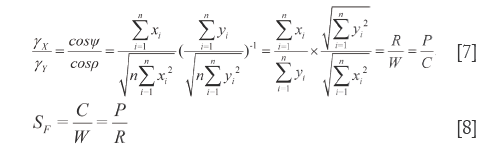
Proposed and intersect at O, the cosine (γX) of the angle (ψ) between = (x1,x2,…,xn) and = [1,1,…,1], the cosine (γY) of angle (ρ) between = (y1,y2,…,yn)and = [1,1,…,1], are calculated to well represent the similar degrees between and or , respectively, thus they are called homogenizing coefficient. The ratio of DQTSs within the 1L-DQTS or 2L-DQTS is just the ratio of γX to γY, see Eq.[7]. We regulate the differences between R and W, P and C not exceeding 15% in order to ensure the distinction of homogenizing coefficient between and less than 15%. In this way, numerical homogeneity degree of any elements of the two vectors is confined to resemblance. Eq.[8] can be derived from Eq.[5] and Eq.[6], which indicates that in general the qualitative similarity is the ratio of two quantitative similarities and merely be used to classify by attribution rather than quantity.
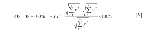
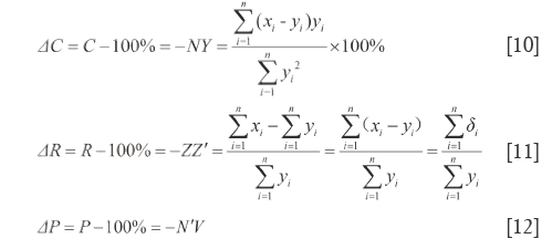
By the respective characteristics, the two level DQTSs compose a tetra-pyramid OXYVZ, see Figure 1. Then change it into a tetra-pyramid OVY X'Z' with a rectangular undersurface (VX'=YZ') and OV=OX'=OY=OZ'=100%. Make XN⊥OY and ZN'⊥OV, connect the lines shown in Figure 1. Module length quantitative QDS (∆W) is deduced on W+XX'=OX'=100%, projection content QDS (∆C) from C+NY=OY=100%, overall content QDS (∆R) from R+ZZ'=OZ'=100% and quantitative QDS (∆P) according to P+N'V=OV=100%, see Eq.[9]-[12]. Above four quantitative similarities W, C, R and P, the higher the errors the bigger the dissimilarities.

 and
and 
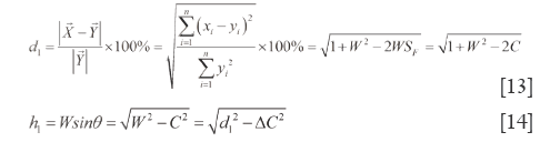
It is generally considered that Euclidean distance is the most famous and convenient to describe the differences between vectors. However, it cannot point out how much in percentage they differ relatively to RV. So Euclidean QDS (d1) is proposed to describe its magnitude relative to RV module length, in which d1 is percentage of - module length to that of to quantitatively reveals how much and differ from each other and with Eq.[13]. The ratio of vertical distance from the vertex of to and the module length is defined as end vertical QDS(h1) as shown in Eq.[14], where it reflects the QDS between and (h1≤d1).
The tetra-pyramid consistes of 4 triangles [1-4] and 3 quadrilaterals [5-7], in which W and R construct the 1L-DQTS in the 4th triange, C and P construct the 2L-DQTS in the 2nd triange. What is more, the lengthes of all lines (in total 17 except 3 replicates) in the hexahedron VYX'Z'NN'XZ can better reflect the quantitative QDS between and , which broaden the quantitative evaluating scope of vectors in n-dimention space.
In the same way, in ∆VOZ and ∆ZON’, because of ZN’⊥OV, Euclidean-liked QDS (d2) and end vertical distance quantitative similarity (h2) are acquired according to R and P. Eq.[15] and Eq.[16] are their formulations (h2<d2).
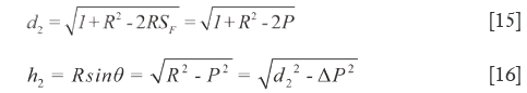
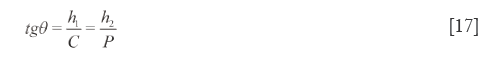
d1, d2, h1, h2 could quantitatively reflect the QDS between and very well (di>hi). When they are equal to zero, and are thoroughly equal. Obviously, tangent value shown as Eq.[17] can qualitatively explain the QDS of and , and is named tangent QDS. The more tgθ is close to zero, the more and are similar in content.
Characteristics of auxiliary rectangular undersurface (the 5th surface)
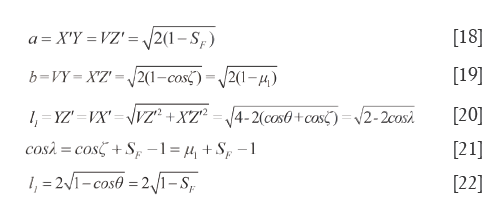
In tetra-pyramid, ∠VOY=∠XOZ=ζ (0≤ζ≤π) and ∠VOX=∠YOZ=λ (θ≤λ≤π), from the rectangular undersurface □VYX’Z’ and cosine theorem, the length of hemline (a) is computed as Eq.[18], the width of hemline (b) is calculated as Eq.[19], and the diagonal length of the undersurface (l1) can be seen in Eq.[20]. Without a doubt, let 0≤ζ≤θ, then a, b and l1 all could reflect the difference degree between SV and RV. When they all trend to zero, the qualitative similarity is the most satisfactory. Let μ1=cosζ, Eq.[21] is derived from Eq.[20], we use Sc=cosλ to reflect the magnitude of similarity between P and W, or between C and R. Because μ1=cosζ is an uncertain value, when ζ=0, b=0 and a=l1; when ζ=θ, a=b, and l1 as displayed in Eq.[22].
Characteristics of quadrilateral undersurface XYVZ (the 6th surface)
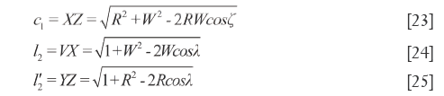
In quadrilateral XYVZ, XY=d1, VZ=d2, VY=b and XZ=c1. According to cosine theorem, the lengths of other sides and the diagonal lengths are respectively measured as shown in Eq.[23]-[25], which also represent the QDS between X and Y. In addition, VX (YZ)> d1 (d2).
Characteristics of quadrilateral section N’NXZ (the 7th surface)
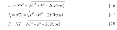
In quadrilateral N'NXZ, NX=h1, N'Z=h2, XZ=c1 and NZ (N'X)>h1 (h2). On the basis of cosine theorem, the lengths of other sides and the diagonal lengths are calculated as displayed in Eq.[26]-[28], which also can disclose the QDS of and .
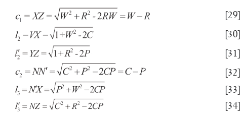
In basic condition of ζ=0, λ=θ the simple and pratical formulars were listed as follow:
In a word, there are 15 parameters for QDS evaluation derived from both 1L-DQTS (W and R) and 2L-DQTS (C and P) to quantitatively assess the difference between and , one of which is closely relevant to Euclidean distance. Their specific applications depend on the existing problems, and must control 0≤ζ≤θ, in which these QDSs can be denoted by percentage. If QSi stands for each sample with the total content similarity, then how much and are quantitatively resemble is represented by QDSi shown in Eq.[35], where tangent DS is the ratio of two quantitative values also belonging to quantitative instinct, and certainly Eq.[35] will give a new QDS method with tgθ. These above new QDSs were summarized in Table 1.

Full table

Application of above QDSs in FLJ quality comparisions
FLJ is the dry flower bud of Lonicera japonica Thunb., with or without young flower (27), which contains chlorogenic acid (CGA), isochlorogenic acid, flavonoids, saponins and volatile oil, etc.. According to the latest statistics by China Economic Forest Association, the annual output of FLJ is 800 million kg in China and its domestic and abroad market demands could be up to 2,000 million kg. Especially during SARS epidemic in 2003, because of good effect of heat-clearing and detoxifying, FLJ had become a shining star of antiSARS and the inventories were once empty. For saling FLJ in the biggest herbal market named Anguo city in Hebei province, China, there were several herbal merchants to become the millionaires over one night, nearly every day emerging one at the period. Though FLJ price had risen over 33 dollars from 3, it is very difficult to buy it. Being so important, we established FLJ-HPLC-FPs to regard the every fingerprint peak area respectively as each element of n-dimentional vector to effectively compared their quality differences by applying above QDSs.
Experimental
Apparatus and reagents
The analysis was performed with an Agilent 1100 HPLC series (Hewlett Packard, CA, USA), consisting of DAD detector, low pressure quaternary pumps, online degasser and an autosampler. All data acquired were proceeded by ChemStation workstation (Agilent technology Inc.). KQ-50B ultrasonic bath (Kunshan ultrasonic instrument company limited, China) and Sarturius-BS110S analytic scale (Saiduolisi scale company limited, Beijing, China) were used during the analysis process. Methanol, acetonotrile (purchased from Yuwang industry limited company, Shandong, China) and glacial acetic acid (provided by Kemiou chemicals developing center, Tianjin, China) were all of HPLC grade. Tetrahydrofuran (THF) of chromatographic grade and ethanol of analytical grade were from Concord Technology Co., Ltd (Tianjin, China). The other reagents were of analytical grade. Deionized water was used for the preparation of all samples and solution. Chlorogenic acid (CGA), Caffeic acid (CFA), and Luteolin (LTL) used as control substances were obtained from National Institute for the Pharmaceutical and Biological Products (Beijing, China) for markers. 3,5-O-dicaffeoylquinic acid (DCQ) was self-made, whose purity was more than 98.6% determined by HPLC. The habitats of 14 batches of raw herbs of FLJs were shown as follows: S1 Linyi, Shandong province; S2 Julu, Hebei province; S3 Hanzhong, Shanxi province; S4 Shangluo, Shanxi province; S5 Baoji, Shanxi province; S6 Xinxiang, Henan province; S7 Pingyi, Shandong province; S8 Feixian, Shandong province; S9 Shandong province, S10 Fengqiu, Henan province; S11 Zhashui, Shanxi province; S12 Wanrong, Shanxi province; S13 Longhui, Hunan; S14 Henan province. All of them were identified by professor Shiyi XU who researches on botany at Shenyang Pharmaceutical University (China) as Lonicera japonica Thunb. except S4, S13 and S14, which were Lonicera confusa DC.
Solution preparation
Control solution
120 µg•mL-1 of CGA was prepared by mixing accurately weighed CGA with 20% methanol, and 150 µg•mL-1 of CFA was also prepared by same method. 680 µg•mL-1 of DCQ was prepared by dissolving accurately weighed in methanol, and 230 µg•mL-1 of LTL was also prepared, all which were stored in refrigerator before use.
Test solution of sample
After being dried under 60 ℃ for 40 min and crushed into powder, 5.0 g of FLJ was weighted accurately. Heat reflux extraction was performed twice with 100 and 60 mL water for 2 h, respectively. The combined filtrate were concentrated to about 20 mL under reduced pressure. Then, ethanol was added to the extracts until its concentration about 80% (v/v). After being stood away from light and kept cool 4 ℃ for 24 h, ethanol was removed completely from the filtrate using a rotary evaporator at 50 ℃. After repeating the alcohol precipitation, the residue was diluted to 50 mL with water and filtered through 0.45 µm microporous membrane before injection.
HPLC conditions
The chromatographic separation was performed on a Century SIL C18 AQ column (250 mm × 4.6 mm, 5 µm) (Dalian Johnsson Separation Science & Technology Corporation, China) at column temperature of (30±0.15) ℃. The mobile phase consisted of binary mixture of solvent A (water, containing 0.5% acetic acid) and solvent B (acetonitrile, containing 5 % THF and 0.5% acetic acid) with a linear gradient program as follows: 0-8 min, 2-5% B; 8-30 min, 5-20% B; 30-60 min, 20-40% B; 60-75 min, 40-50% B. The flow rate was 1.0 mL•min-1 and DAD detector was set at 254 nm, where UV spectra and 3D-plots were recorded between 200 and 400 nm. The injection volume of test solution and control solution were both 5 µL, and eluting time was 75 min.
System suitability tests and selection of reference peak
Five microliters of CGA, CFA, DCQ, LTL and test solution were injected into the chromatograph, respectively, and their chromatograms were recorded as shown in Figure 2. The components thus determined were: peak 9- CGA, peak 11- CFA, peak 21- DCQ. Almost no LTL was detected for its low content in test solution. Because of stronger signal, baseline resolution with the adjacent peaks and moderate retention time, peak 9 was selected as the referential peak (RP), whose theoretical plate number were above 140,000.

Injection precision, sample stability test and method repeatability
Replicately injected the test solution of S10 for 5 times and loaded the test solution of S10 at 0, 1, 5, 15 and 25 h after fresh preparation, respectively, and analyzed 5 independently prepared test solution of S10 to assess the analysis method. All the relative standard deviation (RSD) of relative retention time and of relative peak area were all less than 1% and 3%, respectively, which indicated this method was pretty precise and good in producibility, and stable for test solution within 25 h.
Development of FL-HPLC fingerprint
Respectively, test solutions of S1 to S14 were analyzed and their chromatograms were recorded as shown in Figure 3, in which all fingerprint peaks were eluted within 65 min. Supposed that all the common peaks could be observed in every chromatogram, there were 22 co-possessing peaks marked in the fingerprints. Besides S4, S13 and S14, integral signal of chromatograms was introduced into the professional software named Super-information Characteristic Digitalized Evaluation System for Chromatographic Fingerprints of Traditional Chinese Medicine (Version 4.0), invented by Guoxiang Sun, to yield the referential fingerprint (RFP) by means of average method that synthysized the mean model from S1-S3 and S5-S12 (excluding S4, S13 and S14 due to their lower qualitative similarities), shown in Figure 3 (RFP).

The chromatograms of S4, S13 and S14 significantly differed from those of the rest 11 bathes of FLJ. The various similarities between samples of S1 to S14 and the RFP were calculated as shown in Table 2. SF and SF' of the three batches of Lonicera confusa DC. (S4, S13, S14) were far less than 0.90, thus they were considered as defective goods and could not be regarded as Lonicera japonica Thunb. Although SF of S9 and S12 were more than 0.90, their SF' were less than 0.90 and neither regarded as qualified. Defined ∆SF = SF - SF' and that of S9 and S12 were all above 0.10, which also indicated a bigger discrepancy in the homogenizing coefficient (indicating the uniformity of fingerprint content distribution) γi of the above two samples that were significantly higher than that of RFP. For the 11 batches of FLJs, its |C-P|<12% demonstrated rigorously that they were qualified for their distribution proportion of chemical composition contents with that of RFP. If the mean of the W, R, C, P was denoted as  that was controlled within 70-130%, then the contents of S3, S9, S10 and S12 were outliers that all had the bigger QDSs more than 24. Though the QSs of S4, S13 and S14 were pretty qualified, the qualitative similarities had identified they were not belong to authentical FLJs with the much larger QDSs. According to QDS and DS of samples, S1, S2, S5, S6, S7, S8 and S11 were completely qualified for having the lower QDSs and adequate QSs, in which we calculated the mean of 11 kinds of QDSs in terms of the formular [36] to assess the sample differences. Calculated the mean of d1 and d2; h1 and h2; l2 and l2'; l3 and l3' to be represented by d, h, l2 and l3, respectively, to draw Figure 4 with l1, a and tgθ in order to acquire which is the best QDS parameter.

Full table


Conclusions
Dissimilarity comparision based on vectors in n-dimension space involves overall qualitative similarity and overall quantitative similarity i.e. QSs and QDSs. The d and  were much near furthermore a and tgθ had the closely values. In the present work, several new calculation methods for QDSs had been first set up, which could substitute Euclidean distance to quantitatively reflect the DSs between two n-dimention vectors. Their remarkable characteristics stressed on the differences and compared to QSs in diversity reflected by them were more benefit to classification and evaluation for all things in n-dimentional variances.
The better combination of both the DQLS and the 1L-DQTS or 2L-DQTS could exactly solve the problem of both overall qualitative evaluations and overall quantitative evaluations of all objects with vectors in n-dimension space, in which there 15 QDSs to display the disperity. In a word, the novel QDSs will be getting more important in 21 century for nature and human.
Acknowledgements
This research work was financially supported by National Natural Science Foundation of China (Accession No.90612002) belong to the Important Research Plan “Study on the Scientific Action Circumtances Based on the Internet”, and by Great Projects of the Tenth Five Years Plan granted by Ministry of Science and Technology of China. We also thank National Codex Committee of China for the Funding of the Research Plan of Traditional Chinese Medicine Injection Fingerprints.
Disclosure: The authors declare no conflict of interest.
References
- Sierra G. A simple method for the detection of lipolytic activity of micro-organisms and some observations on the influence of the contact between cells and fatty substrates. Antonie Van Leeuwenhoek 1957;23:15-22.
- Sokal RR, Michener CD. A statistical method for evaluating systematic relationships. Univ Kansas Sci Bull 1958;38:1409-39.
- Jaccard P. Nouvelles recherches sur la distribution florale. Bulletin Société Vaudoise des Sciences Naturelles 1908;44:223-70.
- Jaccard P. Distribution de la flore alpine dans le Bassin des Dranses et dans quelques régions voisines. Bulletin de la Societe vaudoise des Sciences Naturelles 1901;37:241-72.
- Rogers DJ, Tanimoto TT. A Computer Program for Classifying Plants. Science 1960;132:1115-8.
- Pearson K. Mathematical contributions to the theory of evolution - on a form of spurious correlation which may arise when indices are used in the measurement of organs. Proc R Soc London 1897;60:489-502.
- Dice LR. Measures of the amount of ecologic association between species. Ecology 1948;26:297-302.
- Bray JR, Curtis JT. An ordination of the upland forest communities of southern wisconsin. Ecol Monogr 1957;27:325-49.
- Nei M. Estimation of average heterozygosity and genetic distance from a small number of individuals. Genetics 1978;89:583-90.
- Nei M, Li WH. Mathematical model for studying genetical variation in terms of restriction endonucleases. Proc Natl Acad Sci 1979;74:5269-73.
- Zwick R, Carlstein E, Budescu DV. Measures of similarity among fuzzy concepts: A comparative analysis. Int J Approximate Reasoning 1987;1:221-42.
- Ichino M, Yaguchi H. Generalized Minkowski metrics for mixed feature type data analysis. IEEE Trans on Sys Man & Cyb 1994;24:698-708.
- Aitchison J. The statistical analysis of compositional data. J R Stat Soc Ser B 1982;44:139-77.
- Bhattacharya A. On a measure of divergence between two multinomial populations. Sankhyā 1946;7:401-6.
- Ralescu AL, Ralescu DA. Probability and fuzziness. Inf Sci 1984;34:85-92.
- Saraçoğlu R, Tütüncü K, Allahverdi A. A fuzzy clustering approach for finding similar documents using a novel similarity measure. Exp Sys Appl 2007;33:600-5.
- Gowda KC, Diday E. Symbolic clustering using a new dissimilarity measure. Pett Recognit 1991;24:567-78.
- Stephenson W, Williams WT, Cook SD. Computer Analyses of Petersen’s Original Data on Bottom Communities. Ecol Monog 1972;42:387-415.
- Zadeh LA. Fuzzy sets. Inf Control 1965;8:338-53.
- Li RJ. Fuzzy method in group decision making. Comput Math Appl 1999;38:91-101.
- Ölçer Aİ, Odabaşi AY. A new fuzzy multiple attributive group decision making methodology and its application to propulsion/manoeuvring system selection problem. Eur J Ope Res 2005;166:93-114.
- Wang XZ, De Baets B, Kerre E. A comparative study of similarity measures. Fuz Sets Sys 1995;73:259-68.
- Yeh CH, Deng H, Chang YH. Fuzzy multicriteria analysis for performance evaluation of bus companies. Eur J Ope Res 2000;126:459-73.
- Chang YH, Yeh CH. A survey analysis of service quality for domestic airlines. Eur J Ope Res 2002;139:166-77.
- Sun G, Ren P, Bi Y, et al. Fingerprints of ginkgo leaf extract and dipyridamole injection by double qualitative similarities and double quantitative similarities. Se Pu 2007;25:518-23.
- Sun GX, Hou ZF, Zhang CL, et al. Comparison between the qualitative similarity and the quantitative similarity of chromatographic fingerprints of traditional Chinese medicines. Yao Xue Xue Bao 2007;42:75-80.
- Chinese Pharmacopoeia. 2005:I;152.

