Statistical description for survival data
Introduction
Survival analysis encompasses a wide variety of methods for analyzing time-to-event data. In biomedicine, the event of interest may include death, visit to emergency room, myocardial infarction, stroke and intensive care unit (ICU) readmission. The response variable is time. If there is no censoring, traditional regression model can be used to deal with survival data. However, the presence of censoring introduces bias in estimation of survival time distribution. Furthermore, survival data are typically non-negative and positively skewed. Therefore, survival data should be managed with specially designed methods. Instead of focusing on the time (how long) a subject can survive, survival analysis examines the probability of an event at survival time “t” given subjects who are under observation at that survival time. By considering only subjects who are under observation, survival times and survival probability can be estimated without bias given that subjects under observation are representative of the whole study population. A prerequisite assumption is that the censoring mechanism is unrelated to survival time. One scenario that violates this assumption is that when clinical condition deteriorates (e.g., indicating shortened survival time), subjects are more likely to quit a study and they are lost to follow-up. Such censoring is related to survival time. As a result, survival time of subjects who withdraw the study is shorter than those who are still under observation. This is called informative censoring in statistical term.
Here I will not go further into discussion of details and mathematical equation on survival analysis. Instead, I would like to show how survival analysis is performed in R and principles will be introduced with illustrating example. The first article of this theme focuses on statistical description of survival data.
Working example
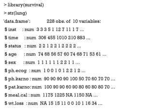
The lung dataset (NCCTG Lung Cancer Data) contained in survival package is employed as working example. This is a dataset containing right-censored survival data.
The dataset contains 228 observations of 10 variables. Institution code (inst) is used to mark different institutions from which patients come. Survival time (time) is measured in days. Censoring status (status) is coded 1 for censored and 2 for dead. Age (age) is measured in years. Male and female sexes are coded as 1 and 2, respectively. ECOG performance score (ph.ecog), Karnofsky performance score rated by physicians (ph.karno) and patients (pat.karno) are also recorded. The last two variables are calories consumed at meals (meal.cal) and weight loss in last six months (wt.loss).
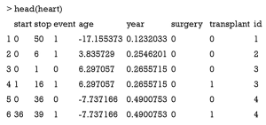
In real world setting, interval censoring can occur when periodic assessments are used to assess if the event of interest has occurred. In this situation, the survival time until an event of interest occurs is not known precisely. Instead, we only have knowledge that the event of interest falls into a particular interval (1,2). The heart dataset (Stanford Heart Transplant data) is a prototype of interval data.
The start and stop variables represent the entry and exit time for an observation period. Note that one subject can take two rows. Age can take negative values because it is centered at 48.
Declaring a survival data
Survival analysis requires to create a survival object using Surv() function. That is equal to declaring a survival data. Survival object is frequently used as response variable in a model formula.
The lung.sur and heart.sur are objects of class Surv. The Surv() takes the general form:
If there are two unnamed arguments as shown in the first line, they will match time and event in that order. If there are three unnamed arguments as that in the second line they match time, time 2 and event. The type argument can usually be omitted.
Nonparametric modeling
Distribution of time-to-event data can be estimated with nonparametric methods such as Kaplan-Meier. The survfit() function can perform this task.
The first argument of survfit() is a formula with the response variable (Surv class object) on the left of the “~” operator. The number “1” on the right indicates a single survival curve. The default type of survival curve is estimated using Kaplan-Meier method. If an object of class “survfit” is passed to the generic function plot(), a survival curve is plotted together with estimated confidence interval (CI) (Figure 1). The default CI is 95%, and it can be customized using conf.int argument in survfit() function. The cross symbol in the figure represents censored observations.
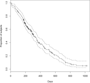
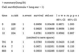
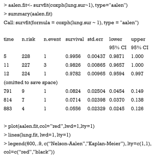
The summary statistics including cumulative survival probability, standard error and 95% CI can be displayed with the following code.
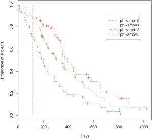
A key feature of the survfit.formula is its ability to fit survival model by strata. The strata are specified by variables on the right of the “~” operator. Factor variables are connected using “+” symbol. For instance, we can compare survival curves by different ECOG performance scores.
In the above example, a variable ph.ecog is added to the right side of “~” operator to make separate survival curves for different ECOG performance score levels. You can try to add sex variable, which will make 8 (2×4) combinations by different values of sex and ECOG performance scores. The argument lty and col assign different line types and colors to distinguish survival curves. Legend() function is used to add annotations (Figure 2).
CIs for the Kaplan-Meier estimator
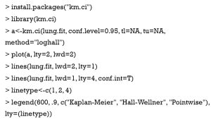
Although the survfit() function allows adjustment of CI for Kaplan-Meier estimator, the underlying method is limited. Here I introduce the km.ci package for computing pointwise and simultaneous CIs for the Kaplan-Meier estimator. Many options exist for computing CI. The method argument allows assigning a string character including “peto”, “linear”, “log”, “loglog”, “rothman”, “grunkemeier”, “hall-wellner”, “loghall”, “epband” and “logep”. In simulation study, Afifi and colleagues found that the Rothman-Wilson (“rothman”), log and Arcsin transformation methods perform better than other methods (3). Confidence band estimation for Kaplan-Meier estimator is an area of active research and comprehensive enumeration of these methods are out of scope of current article. References are provided for interested readers to explore more on this topic (4-8). The following example illustrates how to compute CI.
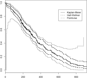
The first argument of km.ci() function is an survival object. The default level of two-sided CI on survival curve is 0.95. Lower (tl) and upper (tu) time boundaries for the simultaneous confidence limits can be specified. If they are missing as in our case, the smallest and largest event times are employed. The Hall-Wellner method is used to compute the confidence bands (9). Figure 3 compares CIs obtained by different methods.
Nelson-Aalen estimator of the survivorship function
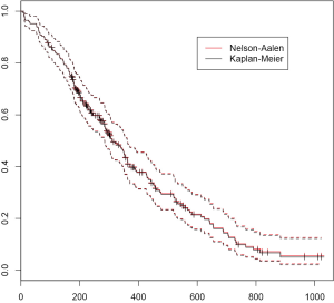
Kaplan-Meier estimator of survival function is the most frequently used estimator, partly because it is the default method in many software packages. Alternatively, survival function can be derived from cumulative hazard function. Nelson and Aalen have proposed an easily computed estimator of cumulative hazard, which is now referred to as Nelson-Aalen estimator (10,11). Nelson-Aalen estimator can be computed via cox regression using coxph() function in R.
The Nelson-Aalen estimator is designated by type=“aalen” argument. Nelson-Aalen estimator of the survival function is always greater than or equal to the Kaplan-Meier estimator (Figure 4). If the size of the risk sets is large relative to the number of events, there will be little practical difference between the Nelson-Aalen and the Kaplan-Meier estimators of the survival function.
Comparison between survival curves
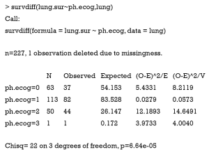
In research practice, an important work is to test whether two survival curves are different based on observed data. In our example, we want to explore whether there is enough reason to reject the null hypothesis that survival curves for lung cancer patients with different ECOG performance scores are similar. Function survdiff() calls a family of tests defined by parameter rho. With ‘rho =0’ it is equivalent to the log-rank or Mantel-Haenszel test, and with ‘rho =1’ it is the Peto & Peto modification of the Gehan-Wilcoxon test (12).
Similar to other survival functions, the first argument of survdiff() function is a formula defining the subgroups to be compared. The left side of the “~” symbol is a Surv class object. If subgroups are defined by combinations of factor variables, they can be connected with “+” operator. The output table shows the observed and expected number of events. The Chi-square statistic for a test of equality shows that the probability of observing current distribution of survival curves is extremely small. Thus, there is enough reason that survival curves are different among subgroups with different ECOG performance scores. If there are two subgroups to be compared, survdiff() performs log-rank test. Otherwise, the function implements statistical test according to the method proposed by Harrington and Fleming (13).
Parametric model
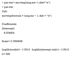
Another way to describe survival data is to assume a mathematical model and then estimate coefficients with maximum likelihood method. Parametric modeling is more appealing in multivariable regression model. For the purpose of statistical description, the intercept only model is employed. Full description of parametric modeling will be introduced in future articles. Here we only take a glimpse of how it works.
The parametric survival model is fit with survreg() function. The first argument is a formula describing the structure of the model. The above code built an intercept-only model and thus “1” is assigned on the right of the “~” symbol. I arbitrarily assumed that T (survival time) follows a Weibull distribution and assigned “w” for the dist argument. Before taking a close look at the output of par.wei, we must review parameters of Weibull distribution.
Let T denotes a continuous non-negative random variable representing survival time. T follows Weibull distribution with parameters lambda (λ) and kappa (κ). The hazard function can be written as Eq. [1]:

and the survival function can be written as Eq. [2]:

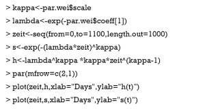
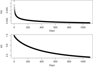
Then the hazard function and survival function can be plotted with a few lines of commands.
The upper panel shows that the hazard h(t) decreases over time (Figure 5). The lower panel shows the survival function, which is comparable to Figure 1. The only distinction is that Figure 1 is depicted with nonparametric method.
Summary
Statistical description is always the first step in data analysis. It gives investigator a general impression of the data at hand. Traditionally, data are described as central tendency and deviation. However, this framework does not fit to the survival data (also termed time-to-event data). Such data type contains two components. One is the survival time and the other is the status. Researchers are interested in the probability of event at a given survival time point. Hazard function, cumulative hazard function and survival function are commonly used to describe survival data. Survival function can be estimated using Kaplan-Meier estimator, which is also the default method in most statistical packages. Alternatively, Nelson-Aalen estimator is available to estimate survival function. Survivor functions of subgroups can be compared using log-rank test. Furthermore, the article also introduces how to describe time-to-event data with parametric modeling.
Acknowledgements
None.
Footnote
Conflicts of Interest: The author has no conflicts of interest to declare.
References
- Radke BR. A demonstration of interval-censored survival analysis. Prev Vet Med 2003;59:241-56. [Crossref] [PubMed]
- Lindsey JC, Ryan LM. Tutorial in biostatistics methods for interval-censored data. Stat Med 1998;17:219-38. [Crossref] [PubMed]
- Afifi AA, Elashoff RM, Lee JJ. Simultaneous non-parametric confidence intervals for survival probabilities from censored data. Stat Med 1986;5:653-62. [Crossref] [PubMed]
- Fay MP, Brittain EH, Proschan MA. Pointwise confidence intervals for a survival distribution with small samples or heavy censoring. Biostatistics 2013;14:723-36. [Crossref] [PubMed]
- Fay MP, Brittain EH. Finite sample pointwise confidence intervals for a survival distribution with right-censored data. Stat Med 2016;35:2726-40. [Crossref] [PubMed]
- Ahmed N, Subramanian S. Semiparametric simultaneous confidence bands for the difference of survival functions. Lifetime Data Anal 2015. [Epub ahead of print]. [PubMed]
- Parzen MI, Wei LJ, Ying Z. Simultaneous Confidence Intervals for the Difference of Two Survival Functions. Scandinavian Journal of Statistics 1997;24:309-14. [Crossref]
- Strobl R, Dirschedl P. S41.5: Comparison of simultaneous and pointwise confidence bands for Kaplan-Meier estimators. Biometrical Journal 2004;46:90. [Crossref]
- Hall WJ, Wellner JA. Confidence bands for a survival curve from censored data. Biometrika 1980;67:133-43. [Crossref]
- Aalen O. Nonparametric Inference for a Family of Counting Processes. The Annals of Statistics 1978;6:701-26. [Crossref]
- Nelson W. Theory and Applications of Hazard Plotting for Censored Failure Data. Technometrics 1972;14:945-66. [Crossref]
- David KG, Mitchel K. Survival Analysis: A Self-Learning Text. Biometrics 2006;62:312. [Crossref]
- Harrington DP, Fleming TR. A class of rank test procedures for censored survival data. Biometrika 1982;69:553-66. [Crossref]


