
Case-crossover design and its implementation in R
Author’s introduction: Zhongheng Zhang, MMed. Department of Critical Care Medicine, Jinhua Municipal Central Hospital, Jinhua Hospital of Zhejiang University. Dr. Zhongheng Zhang is a fellow physician of the Jinhua Municipal Central Hospital. He graduated from School of Medicine, Zhejiang University in 2009, receiving Master Degree. He has published more than 35 academic papers (science citation indexed) that have been cited for over 200 times. He has been appointed as reviewer for 10 journals, including Journal of Cardiovascular Medicine, Hemodialysis International, Journal of Translational Medicine, Critical Care, International Journal of Clinical Practice, Journal of Critical Care. His major research interests include hemodynamic monitoring in sepsis and septic shock, delirium, and outcome study for critically ill patients. He is experienced in data management and statistical analysis by using R and STATA, big data exploration, systematic review and meta-analysis.

Abstract: Case-crossover design is a variation of case-control design that it employs persons’ history periods as controls. Case-crossover design can be viewed as the hybrid of case-control study and crossover design. Characteristic confounding that is constant within one person can be well controlled with this method. The relative risk and odds ratio, as well as their 95% confidence intervals (CIs), can be estimated using Cochran-Mantel-Haenszel method. R codes for the calculation are provided in the main text. Readers may adapt these codes to their own task. Conditional logistic regression model is another way to estimate odds ratio of the exposure. Furthermore, it allows for incorporation of other time-varying covariates that are not constant within subjects. The model fitting per se is not technically difficult because there is well developed statistical package. However, it is challenging to convert original dataset obtained from case report form to that suitable to be passed to clogit() function. R code for this task is provided and explained in the text.
Keywords: Case crossover; R; transient effect; risk ratio; conditional logistic regression; odds ratio
Submitted Mar 23, 2016. Accepted for publication Apr 21, 2016.
doi: 10.21037/atm.2016.05.42
Introduction
Case-control study is a basic study design in epidemiology. It includes all incident cases and a sample of non-cases. Thus, as compared to the cohort study that includes all cases and controls during study period, case-control study is suitable for studying rare disease. However, it is also criticized for its difficulty in controlling between-person confounding (1). Furthermore, case-control study investigates the cumulative effect of an exposure and it is difficult to disentangle acute transient effect from chronic effect. In response to these limitations, the case-crossover design was first developed by Maclure in 1991 (2). The same idea was introduced in a later paper (3). Since then, the case-crossover design has become increasingly popular in medical literature. By searching PubMed in April 2016 [searching strategy: case crossover (title/abstract)], a total of 1,044 citations were identified. The number of publications with case-crossover design increases exponentially in recent years (Figure 1). To assist clinicians become familiar with this design, this paper introduces some basic ideas and rationales behind case-crossover design. R codes for calculations of risk ratio and its variance are present in the main text.

Understanding case-crossover design
Case-crossover design uses all cases for study, and non-cases contribute nothing to the analysis. Because the effect of an exposure is transient, it defines a time window during which the risk of event is transiently elevated. After this window, the risk returns to the baseline level. The history preceding the event of interest is used as the controls. In this regard, case-crossover design can be viewed as matched case control design that controls are the same person before event occurs. Within each person, the person-time of exposure can be estimated by multiplying the frequency of exposure by effect time window. Unexposed person-time can be estimated by subtracting exposed person-time from the total person-time (4). Schematic illustration of the case-crossover design is shown in Figure 2. All patients have the event of interest being observed. All patients have intermittent exposure of risks, and there is a transient effect time window during which the risk is altered. Only patient 2 has the event occurring within the effect time window. In reality, the triggers can be coffee intake, sexual activity, environmental temperature and PM2.5 air pollution. The outcome events can be myocardial infarction (MI), emergency room visit, and intracranial hemorrhage (5-7).

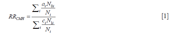
The Cochran-Mantel-Haenszel risk ratio can be written as:
and the Cochran-Mantel-Haenszel odds ratio can be written as:
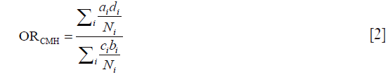
where i is an indicator of the ith stratum, and a, b, c, d, N1, N0 and N are number of participants as shown in Table 1.

Full table
Because each case typically experiences one episode of events, either a or c is equal to 1; and the other is equal to zero. That is, this one episode of event occurs during either exposed or unexposed person-time.
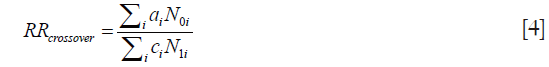
The Cochran-Mantel-Haenszel risk ratio for case crossover study can be written as:
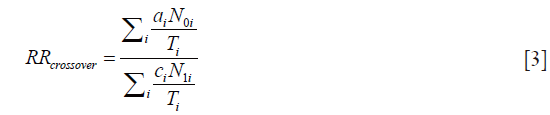
where i is the indicator of the ith case. Either a or c is equal to 1; and the other is equal to zero. N1 is exposed time, and N0 is the unexposed time. T is the total time (Table 2). Because T is typically the same for all participants, it can be eliminated from both numerator and denominator.

Full table
In the case crossover design, we usually know the frequency of trigger activity (frq), total observation time (T), time from last trigger activity to the event (t).
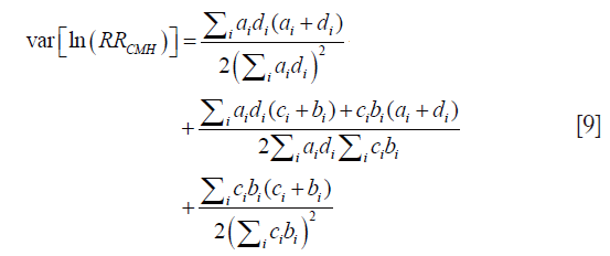
The log variance of Cochran-Mantel-Haenszel RR can be written as (8):
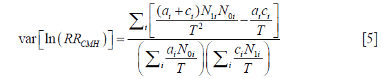
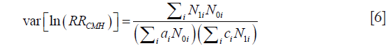
Because either a or c is 0, the last term of the numerator can be eliminated. The T2 can be dropped from numerator and denominator.  is deleted because it equals to one. The equation can be rewritten as:
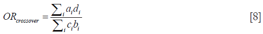
The Cochran-Mantel-Haenszel odds ratio for case-crossover design can be written as:
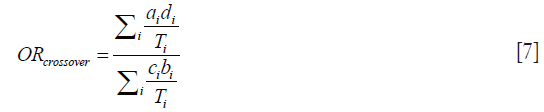
Similarly, this equation can be simplified as:
The log variance of Cochran-Mantel-Haenszel OR can be written as:
Working example
We adapted the study by La Vecchia and colleagues investigating the association between coffee intake and MI (9). It is assumed that the transient effect of coffee lasts for one hour. The variable vectors for ten patients are generated by the following syntax:

The first line generates a variable t, which represents the interval between the last time of coffee intake and MI (hour). The frequency of coffee intake is recorded as counts in the preceding year. The first one has 730 coffee intakes per year, corresponding to twice per day. T is the total number of hours in a year. Vector efftime is a tag variable denoting whether MI occurs within one hour after coffee intake. The last line calculates the risk ratio of MI for periods with coffee effect versus those without coffee effect. Then, we proceed to estimate 95% confidence interval (CI) for RR. The variance in log scale is calculated and then transformed to the original scale.

The Cochran-Mantel-Haenszel OR and its variance can be calculated using the following R syntax:

Conditional logistic regression
Since the case-crossover design can be viewed as matched case-control design with 1:M matched pairs, conditional logistic regression model can be utilized for the estimation of OR of the exposure of interest (4,10). However, the format of data frame described above is not suitable for regression modeling. Therefore the first step is to change the format of data frame, making it suitable for conditional regression analysis. In this example, the clogit() function contained in survival package is employed. The function requires that all person-times, including the exposed and unexposed, be regarded as an observation (e.g., each person-time takes one row). An id variable is used to distinguish between individual patients.

The first line creates a matrix with T-I rows and 0 column. It is an empty matrix. Then I create a for() loop to generate a matrix of exposed and unexposed person-times. In the mat matrix, each column represents one person. Because the first exposed time and its relation to the occurrence of MI are obtained via interview, it is isolated from the mat matrix. The recalled coffee drinking frequency in the preceding year is used to create the mat matrix. There are two kinds of persons. For the first one, the total person-time T is divisible by the exposed person-time (frq). The exposed person time can be equally spaced during the past one year. For the second one, the total person-time T is not divisible by the exposed person-time (frq). The if-else statement is used to do the task.

The above codes combine the person-time matrix with the first interviewed exposure. Then vectors of persons are stacked into one column using melt() function (11). The final data frame contains only thee variables including id, exposure and case. In conditional logistic model, id is used to indicate matched pairs. Here id variable identify persons. The variable exposure denotes exposed [1] and unexposed [0] person-time. The variable case represents the case period and control period. As expected, there is only ten case periods.
The following codes perform conditional logistic regression analysis and its summary output.

The first argument of clogit() function specifies the model structure. Differently from that in generalized linear model, there is a strata argument at the end of the equation. The strata() argument passes the id variable. The output shows that the estimated OR is 1.895 (95% CI: 0.327–10.97), which is similar to that estimated by Cochran-Mantel-Haenszel method.
Time trend adjustment with conditional logistic regression model
Case-crossover design uses subjects as their own control, and thus it is able to eliminate confounding characteristics that are constant within subject. However, there is time trend confounding that cannot be avoided by this method (2). In other words, exposure distribution in any time periods is not globally exchangeable within a person. For example, there is evidence showing that MI risk follows a circadian pattern (12). That is, time periods in the morning are not exchangeable to that at night. Here I create a clock variable to show how to adjust time-varying confounders with conditional logistic regression model.

One day is divided into four clock time periods. Morning (6:00–12:00), afternoon (12:00–18:00), evening (18:00–24:00) and night (0:00–6:00) are denoted by 1, 2, 3 and 4, respectively.

There is a warning message after running the clogit() function. That is because we have no data on the clock time of the occurrence of MI, and I assigned 1 to the clock variable for the first person-time, which is of course not true. However, this doesn’t interfere the illustration of how to adjust time-varying covariates in the model. Risk variance attributable to clock time is expressed by OR.
Summary
Case-crossover design is a variation of case-control design that it employs persons’ history periods as controls. Case-crossover design can be viewed as the hybrid of case-control study and crossover design. Characteristic confounding that is constant within one person can be well controlled with this method. The relative risk and odds ratio, as well as their 95% CIs, can be estimated using Cochran-Mantel-Haenszel method. R codes for the calculation are provided in the main text. Readers may adapt these codes to their own task. Conditional logistic regression model is another way to estimate odds ratio of exposure. Furthermore, it allows for incorporation of other time-varying covariates that are not constant within subjects. The model fitting per se is not technically difficult because there is well developed statistical package. However, it is challenging to convert original dataset from case report form to that suitable to be passed to clogit() function. R code for this task is provided and explained in the text.
Acknowledgements
None.
Footnote
Conflicts of Interest: The author has no conflicts of interest to declare.
References
- Schneeweiss S, Stürmer T, Maclure M. Case-crossover and case-time-control designs as alternatives in pharmacoepidemiologic research. Pharmacoepidemiol Drug Saf 1997;6 Suppl 3:S51-9. [Crossref] [PubMed]
- Maclure M. The case-crossover design: a method for studying transient effects on the risk of acute events. Am J Epidemiol 1991;133:144-53. [PubMed]
- Feldmann U. Epidemiologic assessment of risks of adverse reactions associated with intermittent exposure. Biometrics 1993;49:419-28. [Crossref] [PubMed]
- Mittleman M. Control sampling strategies for case-crossover studies: An assessment of relative efficiency. Am J Epidemiol 1995;142:91-8. [PubMed]
- Weichenthal S, Lavigne E, Evans G, et al. Ambient PM2.5 and risk of emergency room visits for myocardial infarction: impact of regional PM2.5 oxidative potential: a case-crossover study. Environ Health 2016;15:46. [Crossref] [PubMed]
- Weichenthal SA, Lavigne E, Evans GJ, et al. PM2.5 and Emergency Room Visits for Respiratory Illness: Effect Modification by Oxidative Potential. Am J Respir Crit Care Med 2016;193:594-6. [PubMed]
- Zheng D, Arima H, Sato S, et al. Low Ambient Temperature and Intracerebral Hemorrhage: The INTERACT2 Study. Wang X, editor. PLoS One 2016;11:e0149040.
- Rothman KJ, Greenland S, Lash TL, editors. Modern epidemiology. Third, Mid-cycle revision edition. Philadelphia: Lippincott Williams and Wilkins, 2012:758.
- La Vecchia C, Gentile A, Negri E, et al. Coffee consumption and myocardial infarction in women. Am J Epidemiol 1989;130:481-5. [PubMed]
- Marshall RJ, Jackson RT. Analysis of case-crossover designs. Stat Med 1993;12:2333-41. [Crossref] [PubMed]
- Zhang Z. Reshaping and aggregating data: an introduction to reshape package. Ann Transl Med 2016;4:78. [PubMed]
- Takeda N, Maemura K. Circadian clock and the onset of cardiovascular events. Hypertens Res 2016. [Epub ahead of print]. [Crossref] [PubMed]

