Neural networks: further insights into error function, generalized weights and others

Introduction

Neural network (NN) has been introduced in the last article. In this work, more insights will be provided to give readers a comprehensive understanding of how signals are processed in the neural networks. Specifically, key terms and concepts such as error function, generalized weights, multi-layer perceptron and learning rate are illustrated in the working example. I believe that concepts are more comprehensible when they are illustrated in working example than in pure theoretical framework.

Working example

If you have installed MASS package, you can load the birthwt dataset directly into your working space. Otherwise, you need to install MASS package first.

The dataset contains 189 observations and ten variables. The data were collected at Baystate Medical Center, Springfield, Mass during 1986. The first variable is the indicator of low birth weight (low). Mother’s age (age), weight (lwt), race (race), smoking status during pregnancy (smoke), number of previous premature labors (ptl), history of hypertension (ht), presence of uterine irritability (ui), and the number of physician visits during the first trimester (ftv) are recorded. Birth weights of babies are measured and recorded in gram (bwt). The purpose of the study is to predict body weight of newborns with recorded covariates, and body weight has been recorded in gram and as indicator variable. Thus, the outcome can be either binary or continuous.

Training the neural network (NN)

With the help of the neuralnet() function contained in neuralnet package, the training of NN model is extremely easy (1).

The above codes firstly install the neuralnet package and then load it to the working space. The neuralnet() function is powerful and flexible in training a NN model. I leave detailed explanations of its parameters to the next paragraph. After model training, the topology of the NN can be visualized using the generic function plot() with many options for adjusting appearance of the plot. Figure 1 displays topology of the NN. Signal from each of the eight predictors is received by input node. The synaptic weights are displayed above each line. The blue circles indicate bias, corresponding to the intercept in conventional regression model. There is one hidden layer consisting two units. The variable low is output neuron. The total error is 117 and 34 steps are needed for iterations to converge. They are shown at the bottom of the figure.

Figure 1 Visualization of neural network. Signal from each of the eight predictors is received by input node. The synaptic weights are displayed above each line. The blue circles indicate bias, corresponding the intercept in conventional regression model. There is one hidden layer consisting two units. The variable low is output neuron.

The first argument of the neuralnet() function is a formula describing the model to be fitted. As you can see from the example, the specification of the model is similar to that in building generalized linear model (2). The left-hand side specifies the response variable, and the left-hand side is predictors connected by “+” symbols. The “data” argument specifies the data frame on which the NN training is based. The parameter hidden is a vector specifying the number of hidden layers and the number of units in each layer. For example, a vector c(4,2,5) indicates a neural network with three hidden layers, and the numbers of neurons for the first, second and third layers are 4, 2 and 5, respectively. In our example, there is one hidden layer consisting two neurons.

In analogue to the link function in generalized linear model, NN requires to define an activation function. A differentiable activation function can be defined by “act.fct” argument. A string value of “logistic” or “tanh” is acceptable for logistic function or tangent hyperbolicus, respectively. The default is “logistic”. Activation function transforms aggregated input signals, also known as induced local field, into output signal (3). In our example, the output is a binary outcome, and it is left to its default.

The above NN is a multilayer perceptron that contains one or more hidden layers. If a NN contains no hidden layer, it is reduced to the Rosenblatt’s perceptron (4). Other features of a multilayer perceptron include (I) the activation function is differentiable; and (II) the network exhibits a high degree of connectivity.

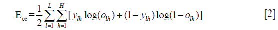
The argument “err.fct” defines the error function, which can be either “sum of squared error (sse)” or “cross entropy (ce)”. The default is “sum of squared error” and it can be expressed as:

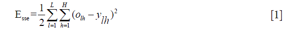
where l=1,2,3,…,L indexes observations, h=1,2,…,H is the output nodes, and o is the predicted output and y is the observed output. Error function in this form is intuitively understandable. However, the comprehension of mathematical expression of cross entropy is a little more challenging:

overall, the error function describes the deviation of predicted outcomes from the observed ones. Large deviation suggests a poorly fitted model and the synaptic weights should be adjusted. The algorithm for NN training is backpropagation. At the very beginning, each synaptic weight adopts a random value. This random model leads to a predicted outcome, which is then compared to the observed outcome. The comparison is made using error function. Absolute partial derivatives of the error function with respect to weight () are slopes used to guide us to find a minimum error (e.g., a slope of zero indicates the nadir).

A new weight () is calculated based on present weight () and the partial derivative.

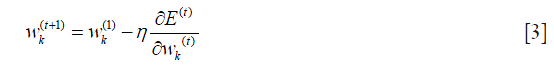
where η is the learning rate, defining the magnitude of weight change in each iteration (3). In traditional backpropagation, the learning rate is fixed, but it can be changed during training process in resilient backpropagation (5,6). Weight update of resilient backpropagation in each iteration is written in the following equation:

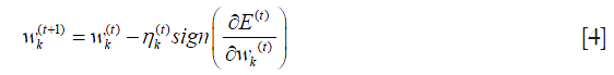
where the learning rate can be changed during training process according to the sign of the partial derivative. The learning rate is increased when the partial derivative keeps its sign. In contrast, if partial derivative of the error function changes its sign, should be decreased. That is because the changing sign suggests the optimal weight is jumped over. Figure 2 is a univariate error function used for illustration. The derivative of error function is negative at step t, then the next weight should be greater than in order to find a weight with a slope equal or close to zero. In reality, because the learning rate is a value greater than 0, the nadir cannot be exactly arrived at but can be approached. Therefore, a threshold should be defined for convergence. By default, the neuralnet() function uses 0.01 as the threshold for partial derivative of error function to stop iteration.

Figure 2 Univariate error function. The derivative of error function is negative at step t, then the next weight should be greater than in order to find a weight with a slope equal or close to zero.

The traditional backpropagation can be performed by assigning “backprop” to the argument “algorithm”. Resilient backpropagation with and without weight backtracking can be specified by “rprop+” and “rprop−”, respectively. Here, weight backtracking is to undo the last iteration and add a smaller value to the weight in the next step. The aim of the technique is to accelerate convergence (1).

Generalized weights

While NN have been proven to have good predictive power as compare to traditional models, its interpretability remains difficult. Interpretability of NN model requires understanding of the independent effect of each individual predictor on the prediction of the model. In 2001, Intrator and coworkers developed the concept of generalized weights for the interpretation of NN (7). The generalized weights are mathematically written as:

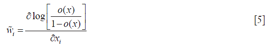
where i is the index for each covariate, o(x) is the predicted outcome probability by covariate vector. Log-odds is the link function for logistic regression model. The partial derivative of the log-odds function with respect to covariate of interest is the coefficient for that covariate. However, if there are non-linear terms for the covariate, generalized weights for that covariate vary greatly over the entire covariate pattern. For linear terms as that in conventional logistic regression model, the generalized weights of a covariate are concentrated at one value. Generalized weights for all observations can be visited in “generalized.weights” element in the nn class object returned by neuralnet() function. Graphical visualization of generalized weights is another way to examine relative contribution of each covariate. The next NN model reduces the number of covariates and increases the number of hidden units.

As you can see from Figure 3, there are four input nodes and four hidden units in the new NN model. With greater degree of freedom, the model reduces the error to 103. However, it requires 18,246 steps for convergence. Complexity of a model is measured by the degree of freedom in conventional models, and increasing complexity carries the risk of model over-fitting (8).

Figure 3 Newly fitted neural network with four input variables. The number of hidden neurons is increased to four. The error of the neural network is reduced to 104, but it requires 18,246 steps for convergence.

The par() function is used to set graphical parameters. After setting mfrow=c(2,2), subsequent figures will be drawn in a 2-by-2 array on the device by rows (mfrow). The gwplot() graphical function is contained in the neuralnet package and it plots general weights against individual covariates (Figure 4). The variances of generalized weights for covariates race and smoke appear large, indicating non-linearity of their effects. If generalized weights of a covariate gather around zero, the covariate has no effect on outcome status.

Figure 4 General weights for each covariate. The variances of generalized weights for covariates race and smoke appear large, indicating non-linearity of their effects.

Prediction with neural network (NN) model

While generalized weights help interpretation of NN model allowing examination of independent effect of covariate, another purpose of NN is to assist prediction of future observations. The model is trained with both input and output signals, which is known as supervised learning in machine learning terminology. For predictions, only input signals are known and they are used to predict outcomes. In our example, suppose we have four months with known feature variables. The probability of having a baby with low birth weight can be calculated with compute() function.

In the above syntax, features of new mothers are stored in a matrix. Note that the order of feature variables should be the same as that in the training data frame. The first argument of the compute() function is the “nn” class object returned by neuralnet(). Next the feature matrix is passed to the function. A list of neurons’ output of each layer and the net results of the neural network are returned by compute() function. Typically, investigators are interested in the final result of the network. As shown in our example, the result shows the probability of having a low birth weight baby for each mother. The first three mothers have 41% probability, and the last one has 5% probability of having a low birth weight baby.

Summary

The article provides further insights into the structure of NN, covering concepts of activation function, error function, learning rate and generalized weights. NN topology can be visualized with generic plot() function by passing a “nn” class object. Generalized weights assist interpretation of NN model with respect to the independent effect of individual input variables. A large variance of generalized weights for a covariate indicates non-linearity of its independent effect. If generalized weights of a covariate are approximately zero, the covariate is considered to have no effect on outcome. Finally, prediction of new observations can be performed using compute() function. Make sure that the feature variables passed to the compute() function are in the same order as that in the training neural network.

Acknowledgements

None.

Footnote

Conflicts of Interest: The author has no conflicts of interest to declare.

References

1. Gunther F, Fritsch S. neuralnet: Training of neural networks. R J 2010;2010:30-8.
2. López-gonzález E. Data analysis from the Generalized Linear Model approach: An application using R | Análisis de datos con el Modelo Lineal Generalizado. Una aplicación con R. Revista Espanola de Pedagogia 2011;69:59-80.
3. Haykin SO. Neural Networks and Learning Machines (3rd Edition). Prentice Hall, 2008.
4. Engel I, Bershad NJ. A transient learning comparison of Rosenblatt, backpropagation, and LMS algorithms for a single-layer perceptron for system identification. IEEE Transactions on Signal Processing 1994;42:1247-51. [Crossref]
5. Riedmiller M. Advanced Supervised Learning in Multi-layer Perceptrons - From Backpropagation to Adaptive Learning Algorithms. Computer Standards & Interfaces 1994;16:265-78. [Crossref]
6. Riedmiller M, Braun H. A Direct Adaptive Method for Faster Backpropagation Learning: The RPROP Algorithm. In IEEE International Conference on Ural Networks 1993:586-91.
7. Intrator O, Intrator N. Interpreting neural-network results: A simulation study. Computational Statistics & Data Analysis 1999;37:373-93. [Crossref]
8. Zhang Z. Too much covariates in a multivariable model may cause the problem of overfitting. J Thorac Dis 2014;6:E196-7. [PubMed]