
Naïve Bayes classification in R
Author’s introduction: Zhongheng Zhang, MMed. Department of Critical Care Medicine, Jinhua Municipal Central Hospital, Jinhua Hospital of Zhejiang University. Dr. Zhongheng Zhang is a fellow physician of the Jinhua Municipal Central Hospital. He graduated from School of Medicine, Zhejiang University in 2009, receiving Master Degree. He has published more than 35 academic papers (science citation indexed) that have been cited for over 200 times. He has been appointed as reviewer for 10 journals, including Journal of Cardiovascular Medicine, Hemodialysis International, Journal of Translational Medicine, Critical Care, International Journal of Clinical Practice, Journal of Critical Care. His major research interests include hemodynamic monitoring in sepsis and septic shock, delirium, and outcome study for critically ill patients. He is experienced in data management and statistical analysis by using R and STATA, big data exploration, systematic review and meta-analysis.

Abstract: Naïve Bayes classification is a kind of simple probabilistic classification methods based on Bayes’ theorem with the assumption of independence between features. The model is trained on training dataset to make predictions by predict() function. This article introduces two functions naiveBayes() and train() for the performance of Naïve Bayes classification.
Keywords: Machine learning; R; naïve Bayes; classification; average accuracy; kappa
Submitted Jan 25, 2016. Accepted for publication Feb 24, 2016.
doi: 10.21037/atm.2016.03.38
Introduction to naïve Bayes classification
Bayes’ theorem can be used to make prediction based on prior knowledge and current evidence (1). With accumulating evidence, the prediction is changed. In technical terms, the prediction is the posterior probability that investigators are interested in. The prior knowledge is termed prior probability that reflects the most probable guess on the outcome without additional evidence. The current evidence is expressed as likelihood that reflects the probability of a predictor given a certain outcome. The training dataset is used to derive likelihood (2,3). Bayes’ theorem is formally expressed by the following equation.

where P(A) and P(B) are probability of events A and B without regarding each other. P(A|B) is the probability of A conditional on B and P(B|A) is the probability of B conditional on A. In naïve Bayes classification, A is categorical outcome events and B is a series of predictors. The word “naïve” indicates that the predictors are independent on each other conditional on the same outcome value. Therefore, which makes the calculation process much easier.
I will use an example to illustrate how the naïve Bayes classification works. The example of sepsis diagnosis is employed and the algorithm is simplified. Suppose there are two predictors of sepsis, namely, the respiratory rate and mental status. Septic patients are defined as fast respiratory rate and altered mental status (4-6). The likelihood table is shown in Table 1. The table is obtained from training dataset. In Bayes’ theorem terms, the likelihood of fast respiratory rate given sepsis is 15/20=0.75, and the likelihood of altered mental status given non-sepsis is 3/80=0.0375. Suppose we have a patient with slow respiratory rate and altered mental status, and we want to make a classification of this patient to either sepsis or non-sepsis.

Full table
The prior probabilities of sepsis and non-sepsis are:
- P(sepsis)=20/100=0.2
- P(non-sepsis)=80/100=0.8
The probabilities of likelihood are:
- P(fast RR|sepsis)=15/20=0.75
- P(slow RR|sepsis)=5/20=0.25
- P(fast RR|non-sepsis)=5/80=0.0625
- P(slow RR|non-sepsis)=75/80=0.9375
- P(altered mental status| sepsis)=17/20=0.85
- P(normal mental status | sepsis)=3/20=0.15
- P(altered mental status|non-sepsis)=3/80=0.0375
- P(normal mental status |non-sepsis)=77/80=0.9625
By applying the maximum a posteriori classification rule (7,8), only the numerator of Bayes’ equation needs to be calculated. The denominators of each classification are the same. The likelihood of sepsis given slow respiratory rate and altered mental status are:
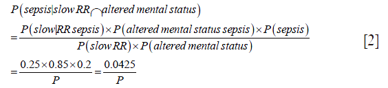
The probability of non-sepsis can be calculated in a similar fashion:
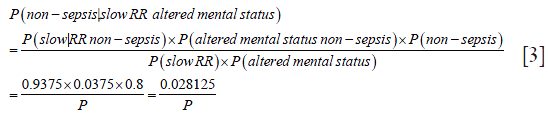
Since the likelihood of sepsis is greater than non-sepsis (0.0425>0.028125), we classify it into sepsis.
Working example
We employed the Titanic dataset to illustrate how naïve Bayes classification can be performed in R.

The dataset is a 4-dimensional array resulting from cross-tabulating 2,201 observations on 4 variables. Because the NaiveBayes() function can pass both data frame and tables, I would like to convert the 4-dimensional array into a data frame with each row represents a passenger. This is also the format with which original data are collected.

The as.data.frame() function converts the array into a data fame with each row representing the unique combinations of all variables. Then the custom-made function countsToCases() (http://www.cookbook-r.com) is employed to expand rows with more than one observations. The new dataset caseTita contains 2201 rows and four columns, which is exactly what we want.
Naïve Bayes classification with e1071 package
The e1071 package contains a function named naiveBayes() which is helpful in performing Bayes classification (9). The function is able to receive categorical data and contingency table as input. It returns an object of class “naiveBayes”. This object can be passed to predict() to predict outcomes of unlabeled subjects.

In the above example, a training model is created by using naiveBayes() function. The model is used to predict the survival status of a random sample of ten passengers. Here we used sample() function to select 10 passengers without replacement. The predicted survival status of them is “No” for nine passengers and “yes” for the last one. If you want to examine the conditional a-posterior probabilities, a character value “raw” should be assigned to the type argument.

The naiveBayes() function receives contingency table as well. The example below is also presented in the help file of the naiveBayes() function.

The a-priori probabilities are prior probability in Bayes’ theorem. That is, how frequently each level of class occurs in the training dataset. The rationale underlying the prior probability is that if a level is rare, it is unlikely that such level will occur in the test dataset. In other words, the prediction of an outcome is not only influenced by the predictors, but also by the prevalence of the outcome. Conditional probabilities are calculated for each variable. It is actually the likelihood table as shown in Table 1. For example, the likelihood of male given survival P(Male|Survived) equals to 0.51617440. Similarly, the predict() function can be applied for new passengers with predictors of age, sex and class.
Naïve Bayes classification with caret package
The caret package contains train() function which is helpful in setting up a grid of tuning parameters for a number of classification and regression routines, fits each model and calculates a resampling based performance measure. Let’s first install and load the package.

Then the data frame caseTita should be split into the predictor data frame and outcome vector. Remember to convert the outcome variable into a vector instead of a data frame. The later will result in error message.

The model is trained by using train() function.

The first argument is a data frame where samples are in rows and features are in columns. The second argument is a vector containing outcomes for each sample. ‘nb’ is a string specifying that the classification model is naïve Bayes. The trainController argument tells the trainer to use cross-validation (‘cv’) with 10 folds. Specifically, the original dataset is randomly divided into 10 equal sized subsamples. Of the 10 subsamples, 9 subsamples are used as training data, and the remaining one subsample is used as the validation data. The cross-validation process is then repeated for 10 times, with each of the 10 subsamples used once as the validation data. The process results in 10 estimates which then are averaged (or otherwise combined) to produce a single estimation (10,11). The output shows a kappa of 0.4, which is not very good. It doesn’t matter since this is only an illustration example. The next task is to use the model for prediction.

The 10 subjects are randomly selected from the original dataset. The first line of the output indicates the row names of the subjects. The second line indicates the survival status by prediction with the model. To compare the predicted results to observed results, a confusion matrix can be useful.

This time the whole dataset was used. It is obvious that the error rate is not low as indicated by off-diagonal numbers.
Summary
The article introduces some basic ideas behind the naïve Bayes classification. It is a sample method in machine learning methods but can be useful in some instances. The training is easy and fast that just requires considering each predictors in each class separately. There are two packages e1071 and caret for the performance of naïve Bayes classification. Key parameters within these packages are introduced.
Acknowledgements
None.
Footnote
Conflicts of Interest: The author has no conflicts of interest to declare.
References
- Efron B. Mathematics. Bayes' theorem in the 21st century. Science 2013;340:1177-8. [Crossref] [PubMed]
- Medow MA, Lucey CR. A qualitative approach to Bayes' theorem. Evid Based Med 2011;16:163-7. [Crossref] [PubMed]
- López Puga J, Krzywinski M, Altman N. Points of significance: Bayes' theorem. Nat Methods 2015;12:277-8. [Crossref] [PubMed]
- Zhang Z, Chen L, Ni H. Antipyretic therapy in critically ill patients with sepsis: an interaction with body temperature. PLoS One 2015;10:e0121919. [Crossref] [PubMed]
- Cohen J, Vincent JL, Adhikari NK, et al. Sepsis: a roadmap for future research. Lancet Infect Dis 2015;15:581-614. [Crossref] [PubMed]
- Drewry AM. Hotchkiss RS1. Sepsis: Revising definitions of sepsis. Nat Rev Nephrol 2015;11:326-8. [Crossref] [PubMed]
- Murphy KP. Machine Learning: A Probabilistic Perspective (Adaptive Computation and Machine Learning series). 1st ed. London: The MIT Press; 2012:1.
- Kononenko I. Machine learning for medical diagnosis: history, state of the art and perspective. Artif Intell Med 2001;23:89-109. [Crossref] [PubMed]
- Misc Functions of the Department of Statistics, Probability Theory Group (Formerly: E1071), TU Wien [R package e1071 version 1.6-7]. Comprehensive R Archive Network (CRAN); 2014. Available online: https://CRAN.R-project.org/package=e1071
- Hadorn DC, Draper D, Rogers WH, et al. Cross-validation performance of mortality prediction models. Stat Med 1992;11:475-89. [Crossref] [PubMed]
- Schumacher M, Holländer N, Sauerbrei W. Resampling and cross-validation techniques: a tool to reduce bias caused by model building? Stat Med 1997;16:2813-27. [Crossref] [PubMed]

